
A Scheduling Strategy for Global Scientific Grids
Minimizing Simultaneously Time and Energy Consumption
Fábio Coutinho
1,2
, Leizer L. Pinto
3
and Cláudio T. Bornstein
4
1
Cosmology and High Energy Physics Laboratory, Brazilian Center for Physics Research – CBPF, Rio de Janeiro, Brazil
2
Computer Institute, Federal University of Alagoas, Maceio, Brazil
3
Informatics Institute, Federal University of Goias, Goiania, Brazil
4
Computer Science and Systems Engineering – PESC, Federal University of Rio de Janeiro – UFRJ, Rio de Janeiro, Brazil
Keywords: Grid Computing, Grid Scheduling, Green Computing, Multiobjective Optimization.
Abstract: Grid computing has consolidated itself as a solution able of integrating, on a global scale, heterogeneous
resources distributed geographically. This fact has contributed significantly to increase the IT infrastructure.
However, all this computer power results in a lot of energy consumption, raising concerns not only with
respect to economic aspects, but also regarding environmental impacts. Current data shows that the
information technology and communication industry has been responsible for 2% of the carbon dioxide
global emission, equivalent to the entire aviation industry. This paper proposes a biobjective strategy for
resource allocation on global scientific grids, considering both energy consumption and execution times. An
algorithm is presented which generates the minimal complete set of Pareto-optimal solutions in polynomial
time. Computation experience is reported for three distinct scenarios.
1 INTRODUCTION
Over the last few years, the scientific community,
enterprise, government and the society at large have
been concerned with environmental issues.
Computers as part of the IT infrastructure affect the
environment in different phases of the product life-
cycle: design, manufacture, operation and disposal.
With respect to the operation of computers, the
energy consumption has been considered as an
important factor of environmental impact
(Murugesan, 2008).
Complex scientific experiments demand high
computing capacity in order to process and store
research data. These experiments consume much
energy by employing large architectures such as
clusters, grids and clouds. For example the Large
Hadron Collider (LHC) (LHC [s.d.]) is a relevant
physics experiment whose computer grid needs
about 2.5MW just for sustaining its major site (tier
0) located at CERN.
Traditionally, in grids, the scheduling of jobs on
machines has been oriented by objectives such as the
minimization of execution times, load balancing and
cache usage. In fact, several studies have explored
grid scheduling aiming at the minimization of the
makespan (Deelman et al., 2004); (Taylor et al.,
2003); (Mcgough et al., 2004). More recently, high-
throughput computing environments have lead task
scheduling studies to consider the reduction of
energy consumption (Beloglazov and Buyya, 2010);
(Orgerie et al., 2008); (Garg and Buyya, 2009);
(Kyong et al., 2007). In a previous work, a heuristic
is proposed in order to reduce the energy
consumption by prioritizing the assignment of
energy-efficient grid resources to the most complex
tasks (Coutinho et al., 2011).
The literature review shows that most papers
either minimize execution times or energy
consumption, i.e. objectives are dealt with
separately. Here we propose the simultaneous
minimization of both energy consumption and
makespan for the grid scheduling problem. This is
attained with the help of BOTEN (BiObjective Time
and ENergy), an algorithm based on multiobjective
optimization techniques.
Several studies in grid scheduling have benefited
from multiobjective optimization techniques
(Camelo et al., 2010); (Zhu et al., 2010); (Garg and
Kumar Singh, 2011); (Talukder et al., 2009).
However, they do not consider the minimization of
energy consumption. In (Miao et al., 2008), a
545
Coutinho F., L. Pinto L. and T. Bornstein C..
A Scheduling Strategy for Global Scientific Grids - Minimizing Simultaneously Time and Energy Consumption.
DOI: 10.5220/0004619905450553
In Proceedings of the 15th International Conference on Enterprise Information Systems (SSOS-2013), pages 545-553
ISBN: 978-989-8565-59-4
Copyright
c
2013 SCITEPRESS (Science and Technology Publications, Lda.)

multiobjective genetic algorithm is presented that
minimizes both execution time and energy
consumption. Nevertheless only a single
multiprocessor system is considered. Berman et al
(Berman et al., 1990) and Bornstein et al (Bornstein
et al., 2012) consider multiobjective optimization for
general combinatorial problems.
The main contributions of this paper are: (i) the
modeling of grid scheduling as a multiobjective
problem; (ii) the development of the BOTEN
algorithm; (iii) a case study illustrating the
scheduling strategy defined by the algorithm; and
(iv) computational results for three distinct
scenarios, considering different variances in the size
of jobs.
The paper is organized as follows. Section 2
describes the grid environment and formulates the
scheduling problem and the corresponding model.
Section 3 presents the BOTEN algorithm, section 4
illustrates the scheduling strategy with an example,
section 5 gives experimental results for three distinct
scenarios and finally section 6 presents the
conclusions.
2 PROBLEM FORMULATION
In this section the execution environment of global
scientific grids is briefly described. Details of the
LHC grid (WLCG, 2002) are given in section 2.1
and the scheduling model is formulated in section
2.2.
2.1 Grid Environment
LHC (LHC [s.d.]) is the world’s largest and highest-
energy particle accelerator. It was built by CERN
(European Organization for Nuclear Research) and
the installations lie in a tunnel of 27 km in
circumference, 175 meters beneath the earth at the
Franco-Swiss border, near Geneva, Switzerland.
Among other things, physicists expect that the LHC
helps to better understand mass structure, particle
characteristics as well as deepen knowledge about
space and time.
In order to fulfill this aim thousands of
researchers in dozens of countries help monitoring
the results of the collisions obtained from the four
main detectors at the LHC: ATLAS, ALICE, CMS
and LHCb. It is estimated that data produced by
these detectors reach approximately 15 petabytes per
year.
The Worldwide LHC Computing Grid (WLCG)
was constructed in order to process this staggering
amount of data and it involves computational centers
of several countries. The CBPF (Brazilian Center for
Physics Research) which is part of the WLCG
contributes mainly in the processing of data from the
LHCb detector. For this purpose the CBPF allocates
a computational infrastructure consisting of two
clusters composed of 65 worker nodes representing a
total capacity of 500 cores. Jobs coming from the
LHCb detector and running at the CBPF are of the
Monte Carlo (MC) type and can take up to two days
of execution time.
The collaboration between CBPF and WLCG
made it possible to observe features of the WLCG
delivering an important motivation for the present
work. As a matter of fact, the huge dimensions of
the grid and its computational infrastructure result in
a high consumption of energy. This fact should be
considered in any study dealing with the
performance of the system.
As already mentioned the WLCG comprises
several geographically distributed sites. These sites
contain heterogeneous machines which process jobs
originating from a meta-scheduler. Each site has a
master/agent architecture for making available the
job scheduling software (batch system like PBS,
Condor, etc.). The scheduling strategy proposed in
this paper aims at helping the meta-scheduler to
decide how jobs are going to be distributed to the
sites of the grid. Some important features of the grid
environment follow:
Grid Load – the number of running jobs depends
on the activity of the detectors. i.e. variation is
great and there are peak loads as seen in Figure 1,
representing the number of jobs generated at
LHCb from March to May 2013.
Availability – sites are required to maintain grid
machines always turned on, i.e. the computational
resources need to be available all the time.
Autonomy – each site manages and controls
independently the corresponding resources. In case
there is no demand from the grid the resources
may be allocated to attend local jobs.
In spite of peak loads (see Figure 1) total amount of
computational grid resources is generally enough to
attend demand generated by the detectors.
Traditionally the meta-scheduler tries to balance the
load so as not to overload the sites of the grid.
The WLCG requirement of the availability of the
machines makes the off-switching of unused CPUs
as a green policy not feasible. Also keeping the local
autonomy makes it difficult to use the DVS
(Dynamic Voltage Scaling) technique at a global
scale as a way of reducing energy consumption
by undervolting. The next section describes the
ICEIS2013-15thInternationalConferenceonEnterpriseInformationSystems
546
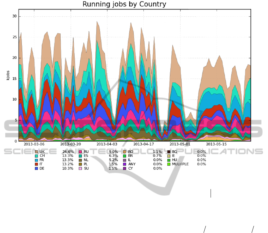
Figure 1: Running jobs from 2013-03-01 to 2013-05-29.
biobjective job scheduling problem.
2.2 Scheduling Model
The problem that will be considered here consists of
a set of n independent jobs that have to be processed
by a grid of m machines. Each machine M
j
has C
j
available cores and C
1
C
2
C
m
≥ n. As a
consequence each job will be allocated to one and
only one core and no core will process more than
one job. As a result, there will be no queuing of jobs.
Not more than C
j
jobs can be allocated to a certain
machine M
j
.
Let
][
ij
xx
for i
=
,,1
n and j
=
,,1
m be the
vector of decision variables representing the
allocation of jobs to machines, i.e.,
1
ij
x
means
that job T
i
is allocated to machine M
j
and
0
ij
x
otherwise. The mathematical model which
represents the biobjective optimization problem is
given by:
12
1
1
minimize ( ) ( ), ( )
subject to: 1, 1, ,
,1,,
0, 1 , 1, , e 1, , ,
m
ij
j
n
ij j
i
ij
Pfxfxfx
xin
xC j m
xinjm
with
}1max{)(
1
ijij
xtxf
and
n
i
m
j
ijij
xexf
11
2
)(
representing makespan and
total energy consumption respectively.
The variables
jiij
SOt
and
jiij
WOe
represent, respectively, the time and the energy
consumption of T
i
processed by a certain core of
machine M
j
. The cores of a certain machine M
j
are
identical. O
i
is the number of floating point
operations of job T
i
. S
j
and W
j
represent the number
of FLOPS and the number of floating point
operations processed per unit of energy (Watt) of a
certain core of machine M
j
respectively. S
j
and W
j
are obtained from benchmarks.
The first objective function
)(
1
xf minimizes the
maximum time spent in execution of the n jobs, i.e.
it minimizes maximum completion time (makespan).
The second objective
)(
2
xf minimizes total energy
consumed by execution of the n jobs.
The first group of restrictions of problem (P)
guarantees that any job will be processed by one and
only one machine of the grid. The second group of
restrictions ensures that no more than C
j
jobs will be
allocated to a machine M
j
.
ASchedulingStrategyforGlobalScientificGrids-MinimizingSimultaneouslyTimeandEnergyConsumption
547

3 THE ALGORITHM
In this section we present the BOTEN algorithm
which solves the problem discussed in the previous
section. Due to the fact that in problem (P) the
objective function is a vector, the problem falls
within vector optimization. Not necessarily there is a
minimum of
)(xf representing an optimal solution.
Therefore it is necessary to work with the weaker
concept of Pareto-optimal solution.
Let
][
ij
xx
and
][
ij
xx
be feasible solutions
of problem (P). x dominates
x
if )()( xfxf and
at least one of the elements of
)(xf is different
from the corresponding element of
)(xf . A
feasible solution x
*
is Pareto-optimal if there is no
other feasible solution that dominates x
*
. A set of
Pareto-optimal solutions X
*
is a minimal complete
set if
xxxfxf ,),()( X
*
and for any Pareto-
optimal solution x
*
there always exists x
X
*
such
that
)()(
*
xfxf .
BOTEN generates a minimal complete set of
Pareto-optimal solutions. The pseudocode of
BOTEN is presented in Figure 2.
The subroutine MinEnergy(
) at line 3 solves
the assignment problem generating a solution
x
that minimizes energy
)(
2
f
subject to the
restriction
)(
1
f
. If no such solution exists we
make
0x . In order to minimize energy, machines
and jobs are ordered in non-increasing values of W
j
and O
i
respectively. MinEnergy(
) first tries to
allocate the biggest job on the machine which
consume least energy (highest value of W
j
). The
algorithm follows in this way until it arrives to the
job with smallest value of O
i
. In order to respect the
restriction
)(
1
f a certain job T
i
is allocated to a
machine M
j
only if
ij
t
. If this is not possible we
follow to the next machine. In case we arrive to the
last machine and we still have
ij
t
we make
0x
. In this case the algorithm terminates and we
make go←0. If
0x
then
)(
2
f
is a minimum under
the restriction
)(
1
f
.
Let us suppose an algorithm that generates non-
decreasing values of
)(
2
f
. At a certain iteration let
solution x result in values
)(
1
xf
and
)(
2
xf
. At the
next iteration let the results be
x
,
)(
1
xf
and
)(
2
xf
.
According to the supposition we have
)()(
22
xfxf
. Then, in order to generate a Pareto- optimal
Figure 2: BOTEN Algorithm.
solution we have to guarantee that )()(
11
xfxf .
This is the rationale that explains procedure
MinEnergy() which is the core idea of the BOTEN
algorithm. Indeed, the iterative process generates
decreasing values of
)(
1
f
and increasing values of
)(
2
f
, guaranteeing that no Pareto-optimal solution
is omitted.
Let us suppose that two feasible solutions x and
x
are generated in two subsequent iterations i and
i+1 respectively. Let us suppose additionally that
0
x . By construction we have )()(
11
xfxf . In
addition we have
)()(
22
xfxf
because at iteration
i+1 the problem handled by MinEnergy() is more
restricted than the similar problem at iteration i. If
)()(
22
xfxf
then certainly x is not Pareto-
optimal and should not be included in set X*. This is
the rationale behind steps 6 and 7 of the algorithm.
BOTEN has polynomial complexity. The number of
iterations is limited by the amount d of different
values of t
ij
. We have
mnd .
. Each iteration results
in running the MinEnergy(
) procedure whose
complexity is
).( mn
because in the worst case we
have to examine all machines for each job. Thus,
complexity of BOTEN is
).()..(
22
mnmnd
.
4 PROBLEM INSTANCE
In order to better discuss the results of the
biobjective formulation, a small example with three
machines (M
1
, M
2
and M
3
) and four jobs (T
1
, T
2
, T
3
and T
4
) is presented. Basic information is given in
the form of a complete bi-partite graph represented
in Figure 3. Each edge (i, j) represents a possible
allocation of job T
i
to machine M
j
.
BOTEN (BiObjective Time and ENergy)
1. X
*
← Ø, go ← 1 and x ← MinEnergy(∞)
2. While (go = 1) Do
3.
x
← MinEnergy(f
1
(x))
4. If (
x
= 0) Then
5. X
*
← X
*
x and go←0
6. Else If (f
2
(x) < f
2
(
x
)) Then
7. X
*
← X
*
x
8. x ←
x
9. End While
End Algorithm
ICEIS2013-15thInternationalConferenceonEnterpriseInformationSystems
548
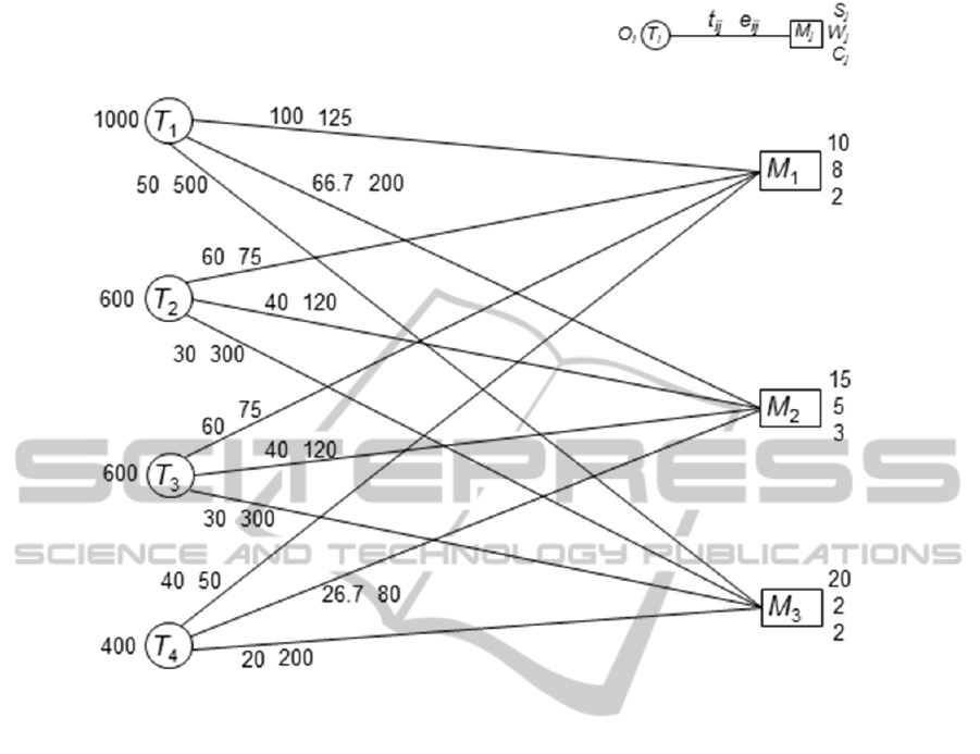
Figure 3: Input data modeled as a complete bi-partite graph.
Figure 4 depicts the four solutions A, B, C and D
generated sequentially by BOTEN. The dashed
edges represent the actual allocation of jobs to
machines.
The first solution A is obtained making
.
Thus, all edges of Figure 3 are considered for
possible allocation of jobs to machines.
MinEnergy(∞) obtains solution A with
1
42322111
xxxx . All other variables are
equal to zero.
400)(
2
Af represents the minimum
possible value of energy consumption while
maximum time completion for all the jobs is
100)(
1
Af
.
The second solution B is obtained by
MinEnergy(100).
100
means, for example,
pruning edge (1, 1), i.e., T
1
cannot be allocated to M
1
and the algorithm allocates T
1
to M
2
. Following in
this way we get solution B with
1
42312112
xxxx
,
430)(
2
Bf
and
7.67)(
1
Bf
. As
)()(
22
BfAf
solution A is
accepted as Pareto-optimal.
Solution C is obtained by MinEnergy(67.7) with
,1
42312113
xxxx
730)(
2
Cf
and
60)(
1
Cf
. As
)()(
22
CfBf
solution B is Pareto-
optimal.
Next iteration solution D is obtained by
MinEnergy(60) with
,1
41322213
xxxx
790)(
2
Df
and
.50)(
1
Df
Solution C is
accepted because
)()(
22
DfCf
. As there is no
possible allocation for MinEnergy(50) the algorithm
terminates accepting D as Pareto-optimal.
BOTEN generates the four Pareto-optimal
solutions out of the 62 feasible solutions. Of course
the decision maker has to make the final decision.
Additional criteria can be developed to help in
making this decision. For example, solution B
represents a decrease of more than 30% of makespan
at the cost of an increase of less than 10% of energy
consumption. Thus, B seems to represent an
improvement of solution A. A similar comment can
be made by comparing solution D with respect to C.
According to this kind of analysis, final decision
should be taken considering just solutions B and D.
Additionally, one could also consider economic
criteria, i.e., for example compare the decreasing
cost of saving energy with the cost of increasing
makespan.
ASchedulingStrategyforGlobalScientificGrids-MinimizingSimultaneouslyTimeandEnergyConsumption
549
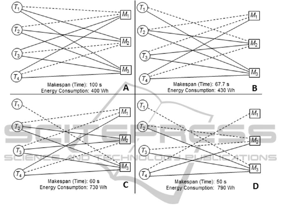
Figure 4: Solutions returned by BOTEN.
5 COMPUTATIONAL
EXPERIMENTS
In this section we present computational results for
BOTEN for the three problems BP1, BP2 and BP3.
Each problem considers 200 jobs processed by 24
machines selected from the Green500 List
(Green500, [s.d.]). Green500 is based on the known
TOP500 List (TOP500 [s.d.]), and ranks the most
energy-efficient supercomputers in the world
(MFLOPS/Watts). Information about machines
considered in the tests, i.e. values of S
j
and W
j
, are
presented in Table 1. As we see, not always the most
energy-efficient resource is the one that minimizes
execution times and vice-versa.
The machines were selected in order to reflect
typical grid heterogeneity. For simplicity, we will
assume that all machines have 16 available cores in
order to process the 200 jobs, i.e.
16
2421
CCC
.
BP1, BP2 and BP3 represent three distinct
scenarios that basically differ in the way numerical
values for the O
i
are generated. BP3 has equal values
for the O
i
, i.e. the jobs are identical. For BP2 and
BP1 values of O
i
are generated randomly but for
BP2 the variation of the number of floating point
operations of the jobs is much smaller than for BP1.
The values of O
i
, S
j
and W
j
allow the calculation
of the e
ij
and t
ij
for each possible allocation of jobs to
machines for the three problems.
BOTEN algorithm was implemented in C
language. The input file contains data for a bi-partite
graph similar to the one presented in Figure 3. The
BOTEN output for each Pareto-optimal solution
consists of two files; the first file gives the
assignment of jobs to machines while the second file
gives the makespan and total energy consumption.
For obvious reasons the following tables present just
data from the second file.
Table 2 presents the results for BP1. The
minimal complete set consists of 96 Pareto-optimal
solutions. For each solution makespan (time) is
given in minutes and energy consumption in kWh.
The corresponding results for BP2 are shown in
Table 3 where the 70 Pareto-optimal solutions of the
minimal complete set are given.
The values of O
i
, S
j
and W
j
allow the calculation
ICEIS2013-15thInternationalConferenceonEnterpriseInformationSystems
550

Table 1: Grid machines considered by the problems.
Green500
Position
W
j
(Mflops/W)
Description
S
j
(Gflops)
1 0.26386 BlueGene/Q 1.60 GHz 22.460156250000
5 0.14563 NNSA/SC Blue Gene/Q P1 5.631420199931
6 0.13922 DEGIMA Cluster, Intel i5 6.203030303030
10 0.00898 HP ProLiant Xeon 6C X5670 16.266819509266
44 0.01798 Cray XE6 Opteron 2.10 GHz 6.519349164468
45 0.02411 Amazon EC2 Cluster 2.60GHz 14.103031015038
75 0.02809 iDataPlex DX360M3, Xeon 2.66 9.465277777778
81 0.05457 Power 775 3.836 GHz 23.090277777778
134 0.05063 HS22, Xeon QC GT 2.66 GHz 9.214089439655
149 0.00113 Cray XT5-HE Opteron 2.6 GHz 7.847003506393
172 0.01934 HS22 Xeon E5649 6C 2.53 GHz 5.635066526611
187 0.01803 HS22 Xeon X5650 6C 2.66 GHz 5.626102564103
208 0.00642 iDataPlex, Xeon E55xx 2.53 GHz 5.575396825397
233 0.01601 x3650M3, Xeon X56xx 2.53 GHz 5.635039641503
244 0.01391 x3550M3 Xeon X5650 2.66 GHz 5.635062748699
275 0.00674 Sun R422, Xeon X5570, 2.93 Ghz 10.447080291971
333 0.00335 Cray XE6 8-core 2.4 GHz 7.873665480427
359 0.01454 x3650M2 Xeon E55xx 2.53 Ghz 5.714657366071
378 0.00942 x3650M2 Xeon E55xx 2.26 Ghz 4.806250000000
386 0.00235 Sun x6275, Xeon X55xx 2.93 Ghz 10.214420358153
413 0.00213 Cray XT3/XT4 5.344430485762
488 0.00311 eServer pSeries p5 575 1.9 GHz 6.205766710354
496 0.00164 Cray XT5 QC 2.4 GHz 7.900763358779
500 0.00237 PowerEdge 1850, 3.6 GHz 5.873226950355
of the e
ij
and t
ij
for each possible allocation of jobs to
machines for the three problems.
BOTEN algorithm was implemented in C
language. The input file contains data for a bi-partite
graph similar to the one presented in Figure 3. The
BOTEN output for each Pareto-optimal solution
consists of two files; the first file gives the
assignment of jobs to machines while the second file
gives the makespan and total energy consumption.
For obvious reasons the following tables present just
data from the second file.
Table 2 presents the results for BP1. The
minimal complete set consists of 96 Pareto-optimal
solutions. For each solution makespan (time) is
given in minutes and energy consumption in kWh.
The corresponding results for BP2 are shown in
Table 3 where the 70 Pareto-optimal solutions of the
minimal complete set are given.
Finally, just four Pareto-optimal solutions were
generated for BP3 whose values (time/energy) are:
89/63208; 87/183096; 85/231576 and 81/244512.
For each table the first solution presents
maximum makespan and minimum energy while the
last solution has the opposite meaning.
For example, for BP2 energy consumption for
the Pareto-optimal solution lies in the [309502,
600485] interval, while makespan ranges in the
[933, 2123] interval. The first solution is
2123/309502 while the last corresponds to
933/600485. As should be expected, decreasing
makespan results in higher energy consumption and
vice-versa. A compromise solution should be found
by the decision maker. For example, the grid meta-
scheduler may choose the median solution or may
try to find the solution with smallest distance to a
fictive minimum 933/309502. Another possibility
would be to find the solution closest to the average
value 1319/405697.
Other aspects related to the problem may also be
considered in the final decision. References and
methods for selecting the final solution can be found
in (Ehrgott and Gandibleux 2002).
6 CONCLUSIONS
This work presents BOTEN, a new scheduling
strategy based on multiobjective optimization for
global scientific grids. The minimization of energy
consumption and makespan are considered
simultaneously. The results show that it is possible
to enhance grid job scheduling with green policies
and still maintain the performance with respect
to execution times. In other words, time and energy
ASchedulingStrategyforGlobalScientificGrids-MinimizingSimultaneouslyTimeandEnergyConsumption
551

Table 2: Solutions of the BP1 Problem.
BP1 Solutions
Sol. Time/Energy Sol. Time/Energy Sol. Time/Energy Sol. Time/Energy Sol. Time/Energy
1 2042/211506 21 1505/223941 41 1209/239971 61 1006/274286 81 868/432036
2 1983/211555 22 1478/224584 42 1197/241222 62 1004/274299 82 863/432666
3 1924/211562 23 1421/225880 43 1194/243476 63 995/290482 83 858/443177
4 1908/211587 24 1397/225914 44 1182/245369 64 994/290843 84 850/443206
5 1894/211682 25 1361/226665 45 1180/246227 65 986/297742 85 845/444018
6 1881/211745 26 1356/226674 46 1176/247341 66 977/312945 86 839/468001
7 1854/211872 27 1290/227476 47 1162/250092 67 968/313179 87 833/473164
8 1827/211998 28 1284/227737 48 1155/251187 68 967/329350 88 828/478680
9 1805/213329 29 1273/230487 49 1154/252677 69 959/354903 89 827/499631
10 1800/213357 30 1268/230499 50 1145/252696 70 951/355128 90 814/503405
11 1776/214086 31 1266/231367 51 1128/254841 71 941/366699 91 806/503721
12 1773/214105 32 1263/232088 52 1102/259921 72 940/366834 92 804/512074
13 1746/215690 33 1250/232160 53 1095/263957 73 933/373004 93 799/517834
14 1720/218495 34 1248/232912 54 1065/263971 74 923/387532 94 796/517858
15 1639/220206 35 1243/235122 55 1049/263997 75 917/387623 95 792/517903
16 1628/221285 36 1236/235131 56 1048/264493 76 916/387643 96 789/529335
17 1612/221319 37 1233/236365 57 1036/267760 77 914/402371
18 1585/221730 38 1230/237050 58 1031/267782 78 898/417743
19 1558/222269 39 1215/238809 59 1021/268233 79 888/428695
20 1532/223262 40 1213/239951 60 1013/273970 80 887/428711
Table 3: Solutions of the BP2 Problem.
BP2 Solutions
Sol. Time/Energy Sol. Time/Energy Sol. Time/Energy Sol. Time/Energy
1 2123/309502 19 1397/351363 37 1233/375456 55 1092/481645
2 2042/309629 20 1370/356767 38 1230/375812 56 1085/492930
3 2015/309851 21 1358/358519 39 1222/376443 57 1056/497944
4 1988/310074 22 1357/358959 40 1215/384001 58 1049/522075
5 1935/310581 23 1356/359140 41 1212/385679 59 1021/523630
6 1908/310898 24 1343/361472 42 1206/386085 60 1018/535842
7 1881/311722 25 1339/365285 43 1197/388914 61 1013/551366
8 1854/312040 26 1321/365420 44 1180/390561 62 1009/555951
9 1773/312640 27 1310/366328 45 1173/390926 63 989/555970
10 1720/313176 28 1303/367223 46 1171/398182 64 986/556550
11 1693/313673 29 1302/367788 47 1162/398595 65 977/585773
12 1666/314657 30 1285/368060 48 1158/402922 66 959/587825
13 1612/317101 31 1284/368935 49 1140/404279 67 957/588496
14 1558/326962 32 1268/370152 50 1133/407218 68 951/589476
15 1505/329113 33 1266/372029 51 1127/421229 69 941/600040
16 1451/343474 34 1250/372796 52 1122/450773 70 933/600485
17 1424/346684 35 1248/374155 53 1121/450776
18 1414/351089 36 1245/375012 54 1109/452643
can be reduced in a balanced way.
BOTEN provides a non-intrusive method (unlike
DVS technique) for reducing power consumption so
as to efficiently allocate resources to scientific grids.
This fact ensures site autonomy in global grid
environment. Benchmark values are used resulting
in more flexibility. Besides, by respecting the upper
limit C
j
of available cores for each machine M
j
, the
algorithm helps the meta-scheduler to balance grid
load.
As discussed in the previous section, BOTEN
was evaluated using three distinct problems. Each
problem represents a different scenario with the
same machines but different sets of jobs. BP1, BP2
and BP3 generated respectively, 96, 70 and 4 Pareto-
optimal solutions.
As expected, the increase in the variation of the
size of the jobs increases the variation of the output
concerning energy consumption and makespan,
decreasing the number of dominated solutions and
ICEIS2013-15thInternationalConferenceonEnterpriseInformationSystems
552

therefore increasing the number of Pareto-optimal
solutions. Indeed, BP1 with the greatest variation in
the size of jobs has the greatest number of Pareto-
optimal solutions while BP3, with all jobs of
identical size, has just four Pareto-optimal solutions.
In future, we intend to evaluate the algorithm for
new scenarios and extend this strategy to cloud
environment. In addition, it would be good to
include also the energy used by disc units in grid
storage in the energy consumption.
ACKNOWLEDGEMENTS
This work was partially supported by CNPq
(Brazilian Science Foundation).
REFERENCES
Beloglazov, A. & Buyya, R., 2010. Energy Efficient
Resource Management in Virtualized Cloud Data
Centers. In Proceedings of the 10th IEEE/ACM
International Conference on Cluster Cloud and Grid
Computing (CCGrid 2010). Melbourne, Victoria, p.
826–831.
Berman, O., Einav, D. & Handler, G., 1990. The
Constrained Bottleneck Problem in Networks.
Operations Research, 38(1), p.178–181.
Bornstein, C.T. et al., 2012. Multiobjective combinatorial
optimization problems with a cost and several
bottleneck objective functions: An algorithm with
reoptimization. Computers & Operations Research,
39(9), p.1969–1976.
Camelo, M., Donoso, Y. & Castro, H., 2010. A Multi-
Objective Performance Evaluation in Grid Task
Scheduling Using Evolutionary Algorithms. In
Proceedings of the Applied Mathematics and
Informatics. Athens, Greece, p. 100–105.
Coutinho, F., de Carvalho, L.A.V. & Santana, R., 2011. A
Workflow Scheduling Algorithm for Optimizing
Energy-Efficient Grid Resources Usage. In
Proceedings of the IEEE Ninth International
Conference on Dependable, Autonomic and Secure
Computing (DASC). Sydney, Australia, p. 642 –649.
Deelman, E. et al., 2004. Pegasus: Mapping scientific
workflows onto the grid. In Proceedings of the 2nd
European across Grids Conference. Cyprus, p. 11–20.
Available at: http://citeseer.ist.psu.edu/viewdoc/
summary?doi=10.1.1.85.4644.
Ehrgott, M. & Gandibleux, X., 2002. Multiple Criteria
Optimization: State of the Art Annotated Bibliographic
Surveys 1st ed., Kluwer Academic Publishers.
Garg, R. & Kumar Singh, A., 2011. Multi-Objective
Optimization to Workflow Grid Scheduling using
Reference Point based Evolutionary Algorithm.
International Journal of Computer Applications,
22(6), p.44–49.
Garg, S. & Buyya, R., 2009. Exploiting Heterogeneity in
Grid Computing for Energy-Efficient Resource
Allocation. In Proceedings of the 17th International
Conference on Advanced Computing and
Communications (ADCOM 2009). Bengaluru, India.
Available at: http://citeseerx.ist.psu.edu/viewdoc/
summary?doi=10.1.1.147.7416 [Accessed May 30,
2013].
Green500, The Green500 List. Available at: http://
www.green500.org/ [Accessed May 30, 2013].
Kyong, H. K., Buyya, R. & Jong, K., 2007. Power Aware
Scheduling of Bag-of-Tasks Applications with
Deadline Constraints on DVS-enabled Clusters. In
Proceedings of the 7th IEEE CCGRID 2007. Seventh
IEEE International Symposium on Cluster Computing
and the Grid, 2007. CCGRID 2007. Rio de Janeiro,
Brazil: IEEE, p. 541–548.
LHC, LHC Project. Available at: http://lhc.web.cern.
ch/lhc/ [Accessed May 30, 2013].
Mcgough, S. et al., 2004. Workflow Enactment in ICENI.
In Proceedings of the UK e-Science All Hands
Meeting. Nottingham, UK, p. 894–900. Available at:
http://citeseerx.ist.psu.edu/viewdoc/summary?doi=10.
1.1.137.4143.
Miao, L. et al., 2008. A Multi-Objective Hybrid Genetic
Algorithm for Energy Saving Task Scheduling in
CMP system. In Proceedings of the IEEE
International Conference on Systems Man and
Cybernetics. Singapore, p. 197–201.
Murugesan, S., 2008. Harnessing Green IT: Principles and
Practices. IT Professional, 10(1), p.24–33.
Orgerie, A.-C., Lefevre, L. & Gelas, J.-P., 2008. Save
Watts in Your Grid: Green Strategies for Energy-
Aware Framework in Large Scale Distributed
Systems. In Proceedings of the 14th IEEE
International Conference on Parallel and Distributed
Systems (ICPADS 2008). 14
th
IEEE International
Conference on Parallel and Distributed Systems, 2008.
ICPADS’08. Melbourne, Australia: IEEE, p.171–178.
Talukder, A.K.M.K.A., Kirley, M. & Buyya, R., 2009.
Multiobjective Differential Evolution for Scheduling
Workflow Applications on Global Grids. Concurrency
and Computation: Practice and Experience, 21(13),
p.1742–1756.
Taylor, I. et al., 2003. Triana Applications within Grid
Computing and Peer to Peer Environments. Journal of
Grid Computing, 1(2), p.199–217.
TOP500, TOP500 Supercomputing Sites. Available at:
http://www.top500.org/ [Accessed May 30, 2013].
WLCG, 2002. Worldwide LHC Computing Grid.
Available at: http://lcg.web.cern.ch/lcg/ [Accessed
May 30, 2013].
Zhu, H. et al., 2010. Grid Independent Task Scheduling
Multi-Objective Optimization Model and Genetic
Algorithm. Journal of Computers, 5(12), p.1907–
1915.
ASchedulingStrategyforGlobalScientificGrids-MinimizingSimultaneouslyTimeandEnergyConsumption
553
