
Flux through a Time-periodic Gate
Monte Carlo Test of a Homogenization Result
Daniele Andreucci, Dario Bellaveglia, Emilio N. M. Cirillo and Silvia Marconi
Department of Basic and Applied Sciences for Engineering, Sapienza University, v.Scarpa 16, 00161 Rome, Italy
Keywords:
Random Walk, Homogenization, Monte Carlo Method, Alternating Pores, Ionic Currents, Cooperating
Evacuees.
Abstract:
We investigate via Monte Carlo numerical simulations and theoretical considerations the outflux of random
walkers moving in an interval bounded by an interface exhibiting channels (pores, doors) which undergo an
open/close cycle according to a periodic schedule. We examine the onset of a limiting boundary behavior
characterized by a constant ratio between the outflux and the local density, in the thermodynamic limit. We
compare such a limit with the predictions of a theoretical model already obtained in the literature as the
homogenization limit of a suitable diffusion problem.
1 INTRODUCTION
A bunch of individuals moves at random inside a
bounded region, say the playground. On the boundary
of the playground there are one or more doors through
which they can exit the playground itself. The time
average flux of individualsexiting the playground will
depend on the local density close to the doors. An in-
teresting question is the following: suppose to know
the rule governing the opening of the doors, what is
the relation between the local individual density close
to the doors and the outgoing flux?
This simple situation models many interesting
phenomena on different space and time scales. We
mention two examples: (i) the playground is a cell,
the individuals are potassium ions, the door is a potas-
sium channel (Hille, 2001; VanDongen, 2004), and
the problem is that of computing the ionic current
through the channel (Andreucci et al., 2011; An-
dreucci et al., 2012). This is a very important question
in biology, indeed ionic channel are present in almost
all living beings and play a key role in regulating the
ionic concentration inside the cells.
(ii) The playground is a smoky room (imagine a
fire in a cinema), the individuals are evacuees, the
door is the door of the room, and the problem is
that of computing at which rate the pedestrian are
able to escape from the room itself (Schadschneider
et al., 2009; Cirillo and Muntean, 2012; Cirillo and
Muntean, 2013). In this case the interesting problem
is that of understanding if the way in which the evac-
uees behave (for instance if they cooperate or not) has
an influence on the outgoing flux magnitude.
In some situations, for instance when the outgo-
ing flux is compensated by an incoming one, a sta-
tionary state with constant (in time) outgoing flux is
achieved. In this case the ratio between the outgoing
flux and the density close to the doors will be, obvi-
ously, a constant, which can be interpreted as the rate
at which the individuals close to the doors succeed to
exit the playground. This situation is also realized on
a short time scale when the number of individuals in
the region is large with respect to the number of them
exiting the doors per unit of time.
A different situation is that in which no incoming
flux is present. In this case the number of individuals
inside the playground decreases and so does the typi-
cal outgoing flux. The natural question is that of un-
derstanding if some time averaged flux has a constant
ratio with respect to the average local density close
to the door (Andreucci and Bellaveglia, 2012). This
question has been posed in (Andreucci and Bellaveg-
lia, 2012) under the assumption that the doors open
with a periodic schedule.
The setup considered in (Andreucci and Bellaveg-
lia, 2012) is very basic and, hence, their result is ab-
solutely general. A scalar field is defined on a d–
dimensional open hypercube where the field evolves
according to the diffusion equation. Homogeneous
Neumann boundary conditions are assumed on the
boundary of the hypercube excepting “small” circles
lying on one of the (d − 1)–hypercubic faces the
626
Andreucci D., Bellaveglia D., N. M. Cirillo E. and Marconi S..
Flux through a Time-periodic Gate - Monte Carlo Test of a Homogenization Result.
DOI: 10.5220/0004620206260635
In Proceedings of the 3rd International Conference on Simulation and Modeling Methodologies, Technologies and Applications (BIOMED-2013), pages
626-635
ISBN: 978-989-8565-69-3
Copyright
c
2013 SCITEPRESS (Science and Technology Publications, Lda.)

boundary is made of. In those circles the boundary
condition is time–dependent on a periodic schedule,
more precisely the positive time axis is subdivided
in disjoint intervals (periodic cycles) of equal length
and any of such intervals is subdived into two disjoint
parts. The boundary condition on the circles is then
assumed to be homogeneous Dirichlet into the first
part of each of these time intervals and homogeneous
Neumann in the second part. (More general shapes
than circles are actually considered in (Andreucci and
Bellaveglia, 2012).)
If the field is interpreted as the density of indi-
viduals in the playgroud, the boundary condition in
(Andreucci and Bellaveglia, 2012) can be described
as follows: the boundary is always reflecting except
for the small circles which are reflecting only in the
second part of each of the time intervals considered
above, while the individuals are allowed to exit the
playground through these circles in the first part of
each of these intervals. In other words the small cir-
cles are doors of the playground and those doors are
open only in the first part of each of the time intervals.
The time periodic micro–structured boundary
conditions suggest to approach the problem from
the homogenization theory point of view (Bensous-
san et al., 1978). With this approach in (Andreucci
and Bellaveglia, 2012) it is proven that, provided the
length of the open time is suitably small with respect
to the length of the cycle, the ratio between the out-
going flux and the field on the small circles (the door)
is not trivial, in the sense that it tends to a real num-
ber when the length of the periodic cycles tends to
zero. This constant ratio is explicitely computed in
(Andreucci and Bellaveglia, 2012) and is proven to
depend on the way in which each time interval is sub-
divided into two parts, that is to say on the length of
the open door and on that of the closed door time sub–
intervals. This result is, in this context, an answer
to the question that opened the paper, namely, to the
question about the relation between the outgoing flux
and the local density of individuals close to the exit.
The present paper has a two–fold aim. In the one–
dimensional case we setup a Monte Carlo simulation
aiming to (i) test numerically the homogenizationlim-
iting result (in the spirit for example of (Haynes et al.,
2010)), (ii) compute the ratio between the outgoing
flux and the local density close to the exit when the
length of the periodic cycles is finite.
This project is realized by introducing a one–
dimensional discrete space model on which indepen-
dent particles perform symmetric random walks. The
space is a finite interval on Z with a boundary point
which is reflecting, whereas the other periodically
changes its status from absorbing to reflecting and
viceversa. We tune the parameters so that the dis-
crete and the continuum space models have equiv-
alent behaviors. Moreover, in the thermodynamics
limit, namely, when the number of site of the discrete
space model tends to infinity, the homogeneization re-
sult proven in the framework of the continuum space
model is recovered. This is not proven rigorously, but
it is demonstrated via heuristc arguments and Monte
Carlo simulations.
The paper is organized as follows. In Sec-
tion 2 we summarize the homogenization results
found in (Andreucci and Bellaveglia, 2012) in the
one–dimensional case. In Section 3 the discrete space
model is introduced and its behavior is discussed on
heuristic grounds. This model is studied via Monte
Carlo simulations in Section 4, where all the numeri-
cal results are discussed. Section 5 is finally devoted
to some brief conclusions.
2 A CONTINUUM SPACE MODEL
In this section we approach the problem via a con-
tinuum space model. We summarize, in the one–
dimensional case, the results found in (Andreucci and
Bellaveglia, 2012). We first introduce the mathemati-
cal model and then discuss its physical interpretation.
Pick the two reals τ ≥ σ ≥ 0, the integer m, and
the function u
0
∈ L
2
([0,L]). Set T = (m + 1)τ and
consider the boundary value problem consisting in the
diffusion equation
u
t
−Du
xx
= 0 on (0,L) ×(0,T) (1)
with D > 0 the diffusion coefficient, the initial condi-
tion
u(x,0) = u
0
(x) ∀x ∈(0,L) (2)
and the boundary conditions
u
x
(0,t) = 0 ∀t ∈[0,T) (3)
and
u(L,t) = 0 ∀t ∈ A and u
x
(L,t) = 0 ∀t ∈C (4)
where
A =
m
τ
[
k=0
[kτ,kτ + σ) and C =
m
τ
[
k=0
[kτ+ σ,kτ+ τ).
According to the discussion in Section 1, the
model above can be interpreted as follows: the field
u is the density of individuals in the playground, m
is the number of the door opening/closing cycles, τ is
the length of each cycle, σ is the length of the time
interval in each cycle during which the door is open,
and, finally, A and C are, respectively, the parts of the
FluxthroughaTime-periodicGate-MonteCarloTestofaHomogenizationResult
627

global time interval [0, T) when the door is open and
closed.
In (Andreucci and Bellaveglia, 2012), via an ho-
mogenization approach, it has been proven the fol-
lowing convergence result in the limit τ → 0 for the
solution of the boundary value problem (1)–(4) pro-
viding an answer to the question about the relation
between the individual density u(L,t) at the door and
the outgoing flux −Du
x
(L,t).
Theorem 2.1. Assume
∃lim
τ→0
√
σ
τ
=: µ ≥ 0 (5)
and let u
τ
be the solution of the boundary value prob-
lem (1)–(4). Then, as τ →0, u
τ
converges in the sense
of L
2
([0,L] ×[0, T)) to the solution u of the problem
(1), (2) with boundary conditions
u
x
(0,t) = 0 ∀t ∈ [0, T) (6)
and
u
x
(L,t) = −
2µ
√
Dπ
u(L,t) ∀t ∈ [0, T) . (7)
Assume
lim
τ→0
√
σ
τ
= ∞; (8)
then the solution of the boundary value problem (1)–
(4) converges to the solution of the problem (1), (2)
with boundary condition
u
x
(0,t) = u(L,t) = 0 ∀t ∈ [0,T). (9)
The physical meaning of the above theorem can
be summarized as follows. If the length τ of each pe-
riodic unit (cycle) is small with respect to
√
σ (see
condition (8)), then, in the τ → 0 limit, the system
behaves as if the door were always open, namely
u(L,t) = 0. On the other hand, if τ is large with re-
spect to
√
σ (see condition (5) with µ = 0), then, in
the τ → 0 limit, the system behaves as if the door
were always closed, namely u
x
(L,t) = 0. Finally,
if τ is of the same order of magnitude of
√
σ (see
condition (5) with µ > 0), then, in the τ → 0 limit,
the system behaves as if the door were open with
the outgoing flux constrained to satisfy the condition
−Du
x
(L,t) = (2µ
p
D/π)u(L,t).
2.1 A Glimpse of the Proof of
Theorem 2.1
In order to explain the mathematical meaning of the
convergence result stated in the theorem, we sketch
the proof of the first part of Theorem 2.1. We refer
the interested reader to (Andreucci and Bellaveglia,
2012) for more details. First of all we note that for
the solution u
τ
of the boundary value problem (1)–(4)
it is not difficult to perform classical energy estimates
and to prove compactness properties in time. Then,
possibly by extracting subsequences, we have that a
function u exists such that as τ → 0
u
τ
converges strongly in L
2
([0,L] ×[0,T)) to u,
and
u
τ
x
converges weakly in L
2
([0,L] ×[0,T)) to u
x
.
Moreover, it is easily proven that u satisfies (1)–(3) in
a standard weak sense. It is important to remark that,
via these simple compactness considerations, it is not
possible to say anything about the limiting boundary
condition satisfied at x = L.
In order to identify such a limiting boundary con-
dition, we consider the weak formulation of problem
(1)–(4). We choose a smooth test function such that
ψ(x,t) = 0 for
x = 0 and t ∈(0,T)
x = L and t ∈ A
x ∈[0, L] and t = T .
By multiplying (1) against ψ and by integrating by
parts we get
−
Z
T
0
Z
L
0
u
τ
ψ
t
+
Z
T
0
Z
L
0
Du
τ
x
ψ
x
=
Z
L
0
u
0
ψ(x,0).
(10)
Next we use the equation above with ψ = ϕw, where
ϕ ∈C
∞
([0,L] ×[0,T]) is such that
ϕ(x,t) = 0 for
x = L and t ∈ (0,T)
x ∈ [0,L] and t = T
and w is chosen as follows.
The choice of the function w is the key ingredi-
ent of the proof. Identifying the properties that the
function w has to satisfy in the setting of alternat-
ing pores is the main point of the paper (Andreucci
and Bellaveglia, 2012), but the general idea of the
definition of w was introduced by (Friedman et al.,
1995) in a stationary case. We consider the interval
I
τ
= (L −
√
Dτ,L) and define w in I
τ
×(0,T) as the
τ–periodic solution of the equation
w
t
+ Dw
xx
= 0 on I
τ
×(0,T) (11)
with boundary conditions
w(L,t) = 0 t ∈ A, w
x
(L,t) = 0 t ∈C,
and, setting for the sake of notational simplicity
X(τ) = L−
√
Dτ,
w(X(τ),t) = 1 t ∈ (0,T).
Notice that we extend w = 1 for x ∈ (0, X(τ)). In
(Andreucci and Bellaveglia, 2012) it is proven that as
τ → 0
w converges strongly to 1 in L
2
((0,L) ×(0,T))
SIMULTECH2013-3rdInternationalConferenceonSimulationandModelingMethodologies,Technologiesand
Applications
628

and
w
x
converges weakly to 0 in L
2
([0,L] ×[0,T)).
Moreover, it is also proven the following highly non–
trivial property: as τ →0
Z
T
0
w
x
(X(τ),t)Du
τ
(X(τ),t)ϕ(X(τ),t) →
−
2µ
√
Dπ
Z
T
0
Du(L,t)ϕ(L,t). (12)
Recall, now, equation (10) and notice that
−
Z
T
0
Z
L
0
u
τ
ϕw
t
+
Z
T
0
Z
L
0
Du
τ
x
w
x
ϕ =
−
Z
T
0
Z
L
0
Du
τ
x
ϕ
x
w+
Z
T
0
Z
L
0
u
τ
ϕ
t
w
+
Z
L
0
u
0
(x)w(x,0)ϕ(x,0)
Since w converges strongly to 1, we get that
−
Z
T
0
Z
L
0
u
τ
ϕw
t
+
Z
T
0
Z
L
0
Du
τ
x
w
x
ϕ
τ→0
−→
−
Z
T
0
Z
L
0
Du
x
ϕ
x
+
Z
T
0
Z
L
0
uϕ
t
+
Z
L
0
u
0
(x)ϕ(x,0).
(13)
We consider next the left hand side in (13) and com-
pute its τ → 0 limit in a different way. First of all we
note that
−
Z
T
0
Z
L
0
u
τ
ϕw
t
+
Z
T
0
Z
L
0
Du
τ
x
w
x
ϕ =
−
Z
T
0
Z
L
0
u
τ
ϕw
t
+
Z
T
0
Z
L
0
D(u
τ
ϕ)
x
w
x
−
Z
T
0
Z
L
0
u
τ
w
x
ϕ
x
.
On the other hand, by using (Du
τ
ϕ) as a test function
for w in (11), and integrating by parts we obtain
−
Z
T
0
Z
L
X(τ)
(Du
τ
ϕ)
w
t
D
+
Z
T
0
Z
L
X(τ)
(Du
τ
ϕ)
x
w
x
=
−
Z
T
0
w
x
(X(τ),t)Du
τ
(X(τ),t)ϕ(X(τ),t).
Recalling, now, that w = 1 for x ∈ (0,X(τ)), from the
two equations above we get
−
Z
T
0
Z
L
0
u
τ
ϕw
t
+
Z
T
0
Z
L
0
Du
τ
x
w
x
ϕ =
−
Z
T
0
w
x
(X(τ),t)Du
τ
(X(τ),t)ϕ(X(τ),t)
−
Z
T
0
Z
L
0
u
τ
w
x
ϕ
x
.
Recalling that w
x
convergesweakly to 0 in L
2
((0,L)×
(0,T)) as τ →0, by (12), the above equality yields
−
Z
T
0
Z
L
0
u
τ
ϕw
t
+
Z
T
0
Z
L
0
Du
τ
x
w
x
ϕ
τ→0
−→
2µ
√
Dπ
Z
T
0
Du(L,t)ϕ(L,t). (14)
By comparing (13) and (14) we finally get
Z
T
0
Z
L
0
[−Du
x
ϕ
x
+ uϕ
t
] +
Z
L
0
u
0
(x)ϕ(x,0)
=
2µ
√
Dπ
Z
T
0
Du(L,t)ϕ(L,t)
which is the weak formulation of the limiting bound-
ary flux condition for u on x = L, given by
Du
x
(L,t) = −
2µ
√
Dπ
Du(L,t) for t ∈ (0,T).
The theoretical approach just sketched will be com-
mented upon also in the Conclusions.
3 A DISCRETE SPACE MODEL
We now approach the problem via a discrete space
model. In this section we first define the model and
then discuss heuristically the relation between the out-
going flux and the individual density close to the door.
This problem will be investigated in the following
section via Monte Carlo simulations.
We consider N one–dimensional independent ran-
dom walkers on Λ = {ℓ,2ℓ,..., nℓ} ⊂ ℓZ and de-
note by t ∈ sZ
+
the time variable. We assume that
each random walk is symmetric, only jumps between
neighboring sites are allowed, that 0 is a reflecting
boundarypoint, and that at the initial time the N walk-
ers are distributed uniformly on the set Λ. Moreover,
we pick the two integers 1 ≤
¯
σ ≤
¯
τ, we partition the
time space sZ
+
in
A =
∞
[
i=1
{s(i−1)
¯
τ,. . . , s[(i−1)
¯
τ+
¯
σ−1]}
and
C =
∞
[
i=1
{s[(i−1)
¯
τ+
¯
σ],.. . ,s[i
¯
τ−1]},
and assume that the boundarypoint (n+1)ℓ is absorb-
ing at times in A and reflecting at times in C.
More precisely, if we let p(x,y) be the probability
that the walker at site x jumps to site y we have that
p(ℓ,ℓ) =
1
2
, p(x,x+ ℓ) =
1
2
for x = ℓ,...,(n−1)ℓ,
FluxthroughaTime-periodicGate-MonteCarloTestofaHomogenizationResult
629

and
p(x,x−ℓ) =
1
2
for x = 2ℓ,...,nℓ;
moreover
p(nℓ,nℓ) =
0 at times in A
1/2 at times in C
and
p(nℓ,(n+ 1)ℓ) =
1/2 at times in A
0 at times in C.
Note that when the walker reaches the site (n+1)ℓ
it is freezed there, so that this system is a model for the
proposed problem in the followingsense: each walker
is an individual, the room is the set Λ = {ℓ,..., nℓ},
at the initial time there are N individuals in the room,
each walker absorbed at the site (n+1)ℓ is counted as
an individual which exited the room. We denote by
P[·] and E[·] the probability and the average along the
trajectories of the process.
In the framework of this model an estimator for
the ratio between the outgoing individual flux and
the typical number of individuals close to the door is
given by
K
i
=
E[F
i
]/(s
¯
τ)
(E[U
i
]/
¯
τ)/ℓ
for all i ∈ Z
+
(15)
where F
i
is the number of walkers that reach the
boundary point (n + 1)ℓ during the i–th cycle, U
i
is
the sum over the time steps in the i–th cycle of the
number of walkers at the site ℓn.
We are interested into two main problems. The
first question that we address is the dependence on
time of the above ratio, in other words we wonder
if this quantity does depend on i. The second prob-
lem that we investigate is the connection between the
predictions of this discrete time model and those pro-
vided by the continuous space one introduced in Sec-
tion 2. These two problems will be discussed in this
section via heuristic estimates and in the next one
via Monte Carlo simulations. Both analytic and nu-
merical computations will be performed under the as-
sumptions
¯
τ ≫
¯
σ and n > 2
¯
σ. (16)
The first hypothesis says that the time interval in
which the right hand boundary point is absorbing is
much smaller than that in which it is reflecting. In
other words in each cycle the door is open in a very
short time subinterval. The second assumption says
that the length of the space interval is larger than 2
¯
σ
and this will ensure that particles being absorbed by
the right hand boundary in a given cycle do not feel
the presence of the left hand endpoint in that cycle.
3.1 The Estimator K
i
is a Constant
Under the first of the two assumptions (16), it is
reasonable to guess that during any cycle the walk-
ers in the system are distributed uniformly in Λ, so
that at each time and at each site of Λ the number
of walker on that site is approximatively given by
E[U
i
]/
¯
τ. Since
¯
σ is much smaller than
¯
τ, the mean
number of walkers E[F
i
] that reach the boundary point
(n+1)ℓ during the cycle i is proportionalto E[U
i−1
]/
¯
τ
and the constant depends only on
¯
σ, so that we have
E[F
i
] =
α(
¯
σ)
¯
τ
E[U
i−1
]. (17)
We also note that, since
¯
τ ≫
¯
σ, we have that
n
1
¯
τ
E[U
i
] = n
1
¯
τ
E[U
i−1
] −E[F
i
]
By combining the two equations above we get that
K
i
= K ≡
h
1
α(
¯
σ)
−
1
n
i
−1
1
¯
τ
ℓ
s
(18)
showing that the estimator (15) does not depend on
time, namely, it is equal to K for each i.
3.2 Estimating α(
¯
σ)
As it will be discussed in the following subsection,
we are interested in finding an estimate for α(
¯
σ) in
the limit
¯
σ large.
First of all we give a very rough estimate of such a
constant. As noted above, since we assumed,
¯
τ ≫
¯
σ,
it is reasonable to imagine that the walkers are dis-
tributed uniformly with density E[U
i−1
]/
¯
τ when the
i–th cycle begins (opening of the door). Hence, since
the walkers are independent, we get
E[F
i
] =
E[U
i−1
]
¯
τ
×S,
where we denote by S the sum over the particles that
at time (i−1)
¯
τ−1 are less than
¯
σ sites from the ab-
sorbing boundary point of the probability that each of
them reaches the absorbing boundary in the next
¯
σ
time steps. Recalling (17), we have
α(
¯
σ) = S. (19)
This representation allows an immediate rough es-
timate of the quantity α(
¯
σ). If
¯
σ is large, at time
¯
σ
each walker space distribution probability can be ap-
proximated by a gaussian function with variance
√
2
¯
σ
(Central Limit Theorem). Hence, the number of par-
ticles that reach in the following
¯
σ steps the boundary
(n + 1)ℓ is approximatively given by the number of
SIMULTECH2013-3rdInternationalConferenceonSimulationandModelingMethodologies,Technologiesand
Applications
630

walkers at the
√
2
¯
σ sites counted starting from the ab-
sorbing boudary point divided by 2. Hence, we find
the estimate
α(
¯
σ) ≈
1
2
√
2
¯
σ =
r
¯
σ
2
suggesting that the quantity α(
¯
σ) depends on
¯
σ as
√
¯
σ.
We now discuss a more precise argument. In or-
der to compute the right hand term in (19) we con-
sider a particle performing a simple symmetric ran-
dom walk on Z and denote by Q the probability along
the trajectories of the process. Since we have assumed
n > 2
¯
σ, see (16), the probability that a particle in the
original model starting at a position which is y site far
from the absorbing boundary point, with 1 ≤ y ≤
¯
σ,
reaches such a point in a time smaller than or equal to
¯
σ is equal to the probability that the single symmet-
ric walker on Z starting at 0 reaches the point y in a
time smaller than or equal to
¯
σ. Then, if we let T
y
be
the first hitting time to y ∈Z for the simple symmetric
walker on Z started at 0, from (19), we have that
α(
¯
σ) =
¯
σ
∑
y=1
Q[T
y
≤
¯
σ] =
¯
σ
∑
y=1
¯
σ
∑
h=y
Q[T
y
= h]
=
¯
σ
∑
y=1
¯
σ
∑
h=y
y
h
Q[S
h
= y]
where S
h
denotes the position of the walker at time h
and in the last equality we have used (Grimmet and
Stirzaker, 2001, Theorem 14 in Section 3.10). Recall-
ing, now, (Grimmet and Stirzaker, 2001, equation (2)
in Section 3.10), we have that
α(
¯
σ) =
¯
σ
∑
y=1
y
¯
σ
∑
h=y:
h+y even
1
h
h
(h+ y)/2
1
2
h
. (20)
We first remark that, since α(
¯
σ) is a double sum
of positive terms, we have that α(
¯
σ) is an increasing
function of
¯
σ. In the next theorem we state two im-
portant properties of α(
¯
σ). The proof of the theorem
will use the result stated in the following lemma.
Lemma 3.1. Let f : Z
+
→ R be a function such that
the limit lim
m→∞
f(m) does exist. Then,
lim
m→∞
1
√
m
m
∑
i=1
1
√
i
f(i) = 2 lim
m→∞
f(m)
Proof. First note that
lim
m→∞
1
√
m+ 1−
√
m
h
m+1
∑
i=1
1
√
i
f(i) −
m
∑
i=1
1
√
i
f(i)
i
= lim
m→∞
1
√
m+ 1−
√
m
f(m+ 1)
√
m+ 1
= 2 lim
m→∞
f(m)
The statement follows by the Stolz-Ces`aro theorem.
Theorem 3.2. The function α : Z
+
→ R satisfies
lim
r→∞
α(r)
√
r
=
r
2
π
. (21)
Proof. We assume r even; the case r odd can be
treated similarly. In order to get (21) we rewrite (20)
as
α(r) = α
e
(r) + α
o
(r) (22)
with
α
e
(r) ≡
r/2
∑
k=1
(2k)
r/2
∑
s=k
1
2s
2s
(2s+ 2k)/2
1
2
2s
and
α
o
(r) ≡
r/2
∑
k=1
(2k−1)
×
r/2
∑
s=k
1
2s−1
2s−1
(2s+ 2k−2)/2
1
2
2s−1
We shall prove that
lim
r→∞
α
e
(r)
√
r
=
r
1
2π
; lim
r→∞
α
o
(r)
√
r
=
r
1
2π
(23)
and hence (22) will imply (21).
We are then left with the proof of (23). We only
prove the first of the two limits; the argument leading
to the second one is similar. First of all we note that
α
e
(r) =
r/2
∑
k=1
r/2
∑
s=k
k
s
2s
s+ k
1
2
2s
=
r/2
∑
s=1
s
∑
k=1
k
s
2s
s+ k
1
2
2s
=
r/2
∑
s=1
2s
∑
h=s+1
h−s
s
2s
h
1
2
2s
Thus, by using the properties of the binomial coeffi-
cients we get
α
e
(r) = −
r/2
∑
s=1
2s
∑
h=s+1
2s
h
1
2
2s
+
r/2
∑
s=1
2s
∑
h=s+1
h
s
2s
h
1
2
2s
= −
r/2
∑
s=1
2s
∑
h=s+1
2s
h
1
2
2s
+
r/2
∑
s=1
2s
∑
h=s+1
2s−1
h−1
1
2
2s−1
and, hence,
α
e
(r) = −
r/2
∑
s=1
2s
∑
h=s+1
2s
h
1
2
2s
+
r/2
∑
s=1
2s−1
∑
ℓ=s
2s−1
ℓ
1
2
2s−1
FluxthroughaTime-periodicGate-MonteCarloTestofaHomogenizationResult
631

Now, by the Newton’s binomial theorem we get
α
e
(r) =
r/2
∑
s=1
n
−
1
2
h
1−
1
2
2s
2s
s
i
+
1
2
o
=
r/2
∑
s=1
1
2
2s+1
2s
s
(24)
which is a notable expression for α
e
. The Stirling’s
approximation finally yields
α
e
(r) =
r/2
∑
s=1
1
2
2s+1
2
2s
1
√
π
1
√
s
[1+ g(s)]
=
1
2
√
π
r/2
∑
s=1
1
√
s
[1+ g(s)]
where g(s) → 0 as s →∞. Hence,
lim
r→∞
α
e
(r)
√
r
=
1
2
√
π
lim
r→∞
1
√
r
r/2
∑
s=1
1
√
s
[1+ g(s)]
=
1
2
√
2π
lim
t→∞
1
√
t
t
∑
s=1
1
√
s
[1+ g(s)] (25)
The first of the two limits (23) finally follows from
(25) and Lemma 3.1.
Moreover, also relying upon the numerical simu-
lations, we conjecture that there exists a positive inte-
ger r
0
such that
α(r+ 1)
√
r+ 1
−
α(r)
√
r
> 0 (26)
for any integer r ≥ r
0
.
3.3 Comparison with the Continuum
Space Model
In order to compare the results discussed above in
this section with those in Section 2 referring to the
continuous space model defined therein, we have to
consider two limits. The parameter
¯
σ has to be taken
large (recall, also, that we always assume
¯
τ ≫
¯
σ, see
(16)) so that, due to the Central Limit Theorem, the
discrete and the continuous space model have similar
behaviors provided the other parameters are related as
2Ds = ℓ
2
. With this choice of the parameters, then, we
expect that, provided the ratio σ/τ
2
is chosen prop-
erly, the discrete space model will give results similar
to those predicted by the continuous space one with
finite τ.
In (Andreucci and Bellaveglia, 2012), see Theo-
rem 2.1, the relation between the outoing flux and the
density close to the pore is worked out only in the
limit τ → 0. We then have to understand how to im-
plement such a limit in our discrete time model.
We perform this analysis in the critical case σ =
µ
2
τ
2
. In order to compare the discrete and the contin-
uum space models we first let
ℓ =
L
n+ 1
. (27)
As already remarked above, from the Central Limit
Theorem, it follows that the two models give the same
long time predictions if 2Ds = ℓ
2
; hence, the time unit
is set to
s =
ℓ
2
2D
=
L
2
2D(n+ 1)
2
. (28)
We then consider the random walk model introduced
above by choosing
¯
σ and
¯
τ such that the equality
¯
σs =
(µ
¯
τs)
2
is satisfied as closely as possible (note that
¯
τ
and
¯
σ are integers). This can be done as follows: we
fix L, n, µ, and
¯
σ and we then consider
¯
τ =
1
µ
r
¯
σ
s
=
1
µ
n+ 1
L
√
2D
¯
σ−δ (29)
where ⌊·⌋ denotes the integer part of a real number
and δ ∈ [0,1]. With the above choice of the parame-
ters, the behavior of the random walk model has to be
compared with that of the continuum space model in
Section 2 with period
τ = s
¯
τ =
1
µ
L
√
¯
σ
(n+ 1)
√
2D
−
L
2
2D(n+ 1)
2
δ. (30)
The equation (30) is very important in our compu-
tation, since it suggests that the homogenization limit
τ → 0 studied in the continuum model should be cap-
tured by the discrete space model via the thermody-
namics limit n →∞. We then expect that the estimator
K has to converge to the constant 2µ
√
D/
√
π in this
limit.
This seems to be the case if we use the heuristic
estimate of the constant K obtained above. Indeed, by
(18) and (30), we have that
K =
1
α(
¯
σ)
−
1
n
−1
r
2D
¯
σ
µ
×
1+
δµL
√
2D
¯
σ
1
n+ 1
+ o
1
n+ 1
(31)
for the ratio between the outgoing flux and the lo-
cal density close to the door, where o(1/(n+ 1)) is
a function tending to zero faster than 1/(n+ 1) in the
limit n → ∞. In the next section we shall obtain such
an estimate via a Monte Carlo computation, but here,
by using (21), we get that
K
n→∞
−→
α(
¯
σ)
√
¯
σ
√
2Dµ
¯
σ→∞
−→
r
2
π
√
2Dµ = 2µ
r
D
π
which is the desired limit.
SIMULTECH2013-3rdInternationalConferenceonSimulationandModelingMethodologies,Technologiesand
Applications
632
4 MONTE CARLO RESULTS
In this section we describe the Monte Carlo computa-
tion of the constant (15). This measure is quite diffi-
cult since in this problem the stationary state is triv-
ial, in the sense that, since there is an outgoing flux
through the boudary point (n + 1)ℓ and no ingoing
flux is present, all the particles will eventually exit
the system itself.
Our problem can be rephrased as follows: both
the outgoing flux and the local density at the door are
two “globally decreasing” random variables, but their
mutual ratio is constant in average. We then have to
set up a procedure to capture this constant ratio.
For the time length of the open state, we shall con-
sider the following values
¯
σ = 30,50, 70,100,120,150,200.
For each of them, in order to perform the limit τ → 0,
we shall consider
n = 200, 400,600, 800,1000,1500,3000,5000,10000
for the number of sites of the lattice Λ.
For each choice of the two parameters
¯
σ and n we
shall run the process and compute at each cycle i the
quantity
k
i
=
F
i
/(
¯
τ)
U
i
/(
¯
τ)
where, we recall,
¯
τ is defined in (29) and F
i
and U
i
have been defined below (15).
0.00018
0.0002
0.00022
0.00024
0.00026
0.00028
0 100 200 300 400 500 600
outgoing ux/local density
cycle
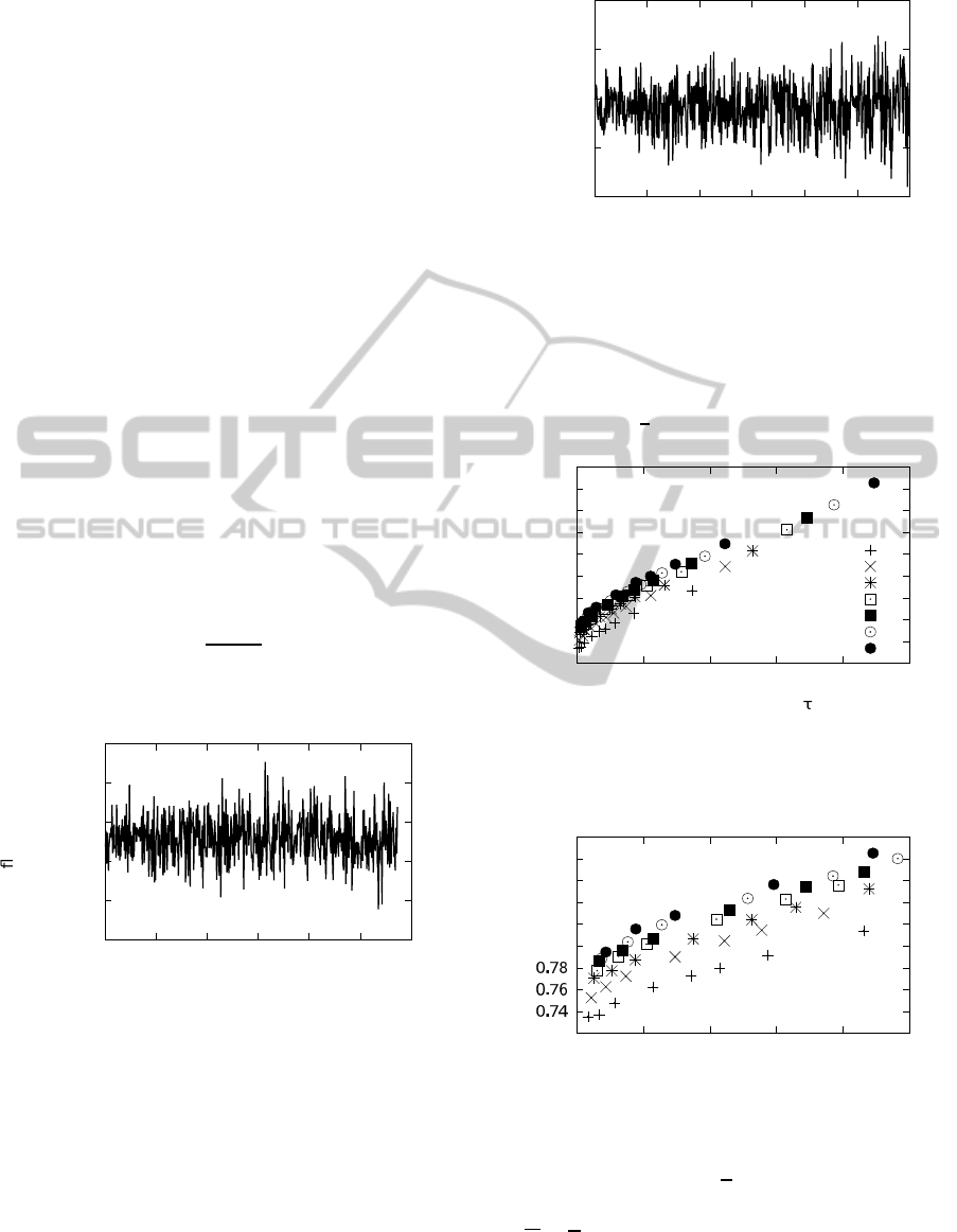
Figure 1: The quantity k
i
is plotted vs. the cycle number i
in the case
¯
σ = 30 and n = 5000.
The quantity k
i
is a random variable fluctuating
with i, but, as it is illustrated in the Figures 1 and 2, it
performs random oscillations around a constant refer-
ence value. We shall measure this reference value by
computing the time average of the quantity k
i
. We
shall average k
i
by neglecting the very last cycles
which are characterized by large oscillations due to
the smallness of the number of residual particles in
the system.
The product of the reference value for the ran-
dom variable k
i
and the quantity ℓ/s, see the equations
0.00022
0.00024
0.00026
0.00028
0.00030
0 100 200 300 400 500 600
outgoing flux/local density
cycle
Figure 2: The quantity k
i
is plotted vs. the cycle number i
in the case
¯
σ = 200 and n = 5000.
(15), (27) and (28), will be taken as an estimate for K.
In other words the output of our computation will be
the quantity
K =
ℓ
s
×(k
i
time average). (32)
0.7
0.75
0.8
0.85
0.9
0.95
1
1.05
1.1
1.15
0 0.05 0.1 0.15 0.2 0.25
constant K
periodic schedule
30
50
70
100
120
150
200
Figure 3: The Monte Carlo estimate of the constant K mea-
sured as in (32) vs. the periodic time schedule τ. Each series
of data refers to the
¯
σ value reported on the right bottom part
of the figure.
0.72
0.8
0.82
0.84
0.86
0.88
0.9
0 0.01 0.02 0.03 0.04 0.05
constant K
periodic schedule τ
Figure 4: The same data as in figure 3 zoomed in the interval
[0,0.05].
We perform the computation described above with
D = 1, L = π, µ = 1/
√
2; with this choice the
continuum space model prediction for the ratio is
2µ
√
D/
√
π = 0.798.
Our numerical results are illustrated in Figures 3
and 4. We note that by increasing
¯
σ the numeri-
cal series tend to collapse to one limiting behavior.
FluxthroughaTime-periodicGate-MonteCarloTestofaHomogenizationResult
633

Table 1: The parameter τ, computed via (30), for the specified values of
¯
σ and n.
n
200 400 600 800 1000 1500 3000 5000 10000
¯
σ
30 0.0865 0.0431 0.0287 0.0215 0.0172 0.0115 0.0057 0.0034 0.0017
100 0.1579 0.0787 0.0524 0.0393 0.0314 0.0210 0.0105 0.0063 0.0031
200 0.2233 0.1114 0.0742 0.0556 0.0445 0.0296 0.0148 0.0089 0.0044
Table 2: Measured constant K for the specified values of
¯
σ and n.
n
200 400 600 800 1000 1500 3000 5000 10000
¯
σ
30 0.8660 0.8140 0.7916 0.7794 0.7723 0.7624 0.7476 0.7371 0.7351
100 1.0059 0.9099 0.8772 0.8559 0.8430 0.8245 0.8017 0.7906 0.7772
200 1.1135 0.9738 0.9269 0.8994 0.8852 0.8564 0.8280 0.8155 0.7944
This is in agreement with what we proved in Sec-
tion 3.2. Moreover, provided
¯
σ is large enough, for
τ → 0 the measured constant tends to the theoretical
value 0.798. For
¯
σ = 30,100,200 we have also re-
ported in Tables 1 and 2 the data plotted in Figure 3.
We can finally state that the Monte Carlo measure
of the constant K is in very good agreement with the
theoretical predictions discussed above.
We also note that, both the continuum space study
outlined in Section 2 and the heuristic discussion of
its discrete space counterpart given in Section 3 were
just able to predict the value of the constant K in the
limit τ →0. No information was given on its behavior
at finite τ.
The Monte Carlo computations, on the other hand,
suggest that K increases with the periodic schedule τ.
We cannot give, at this stage of our reasearch, a phys-
ical interpretation of this result. This is for sure a very
interesting point in the framework of this problem, in-
deed, it is connected with the efficiency of the evacu-
ation phenomenon in connection with the periodicity
of the open/close door cycles.
5 CONCLUSIONS
We have studied via Monte Carlo simulations the out-
going flux through a “door” periodically alternating
between open and closed states. We have shown that
the discrete space random walk model exhibits the on-
set of the same limiting behavior as the continuum
space model sketched in Section 2. The homogeniza-
tion limit of the continuum space model corresponds
to the thermodynamics limit in the discrete space one.
The first one of the goals stated in the Introduc-
tion, that is the numerical test of the homogeniza-
tion result, has been in our opinion achieved (see the
Figures and the comments in Section 4). We remark
that we raised some problems in the theory of random
walk which, albeit not tackled in this paper, seem to
deserve a theoretical investigation (see Section 3.1).
As to our second goal of investigating the prob-
lem for finite τ, we have found clear evidence of a
monotonic behavior in τ of the estimator K, which we
deem believable in view of the just commented co-
herence shown by the Monte Carlo method with the
theoretical Theorem 2.1.
In this connection we must remark that even from
the short account of the main steps in the proof of
Theorem 2.1, given in Section 2.1, it is quite clear that
the monotonic behavior identified by the Monte Carlo
approach is not easily amenable to investigation, or
even discovery, by means of that theoretical approach.
As remarked in the previous Section, we do not
presently providea full insight in the origin and mean-
ing of this behavior, which however is connected with
our conjecture (26), and with the efficiency of the
evacuation phenomenon as a function of τ. It is im-
portant to recall, finally, that at least in biological ap-
plications the efficiency of this mechanism is not the
only concern. For example the alternating schedule
of ion channels has been connected to the selection of
a preferred ion species (VanDongen, 2004). Thus in
general we expect τ to satisfy several different con-
straints coming from different features of the biologi-
cal system.
REFERENCES
Andreucci, D. and Bellaveglia, D. (2012). Permeability
of interfaces with alternating pores in parabolic prob-
lems. Asymptotic Analysis, 79:189–227.
Andreucci, D., Bellaveglia, D., Cirillo, E. N. M., and
Marconi, S. (2011). Monte carlo study of gating
and selection in potassium channels. Phys. Rev. E,
84(2):021920.
Andreucci, D., Bellaveglia, D., Cirillo, E. N. M., and Mar-
coni, S. (2012). Monte carlo study of gating and selec-
tion in potassium channels. preprint arXiv 1206.3148.
SIMULTECH2013-3rdInternationalConferenceonSimulationandModelingMethodologies,Technologiesand
Applications
634

Bensoussan, A., Lions, J. L., and Papanicolaou, G. (1978).
Asymptotic Analysis for Periodic Structures. North
Holland, Amsterdam.
Cirillo, E. N. M. and Muntean, A. (2012). Can cooperation
slow down emergency evacuations? Comptes Rendus
Mecanique, 340(9):625 – 628.
Cirillo, E. N. M. and Muntean, A. (2013). Dynamics of
pedestrians in regions with no visibility – a lattice
model without exclusion. Physica A. In press.
Friedman, A., Huang, C., and Yong, J. (1995). Effective
permeability of the boundary of a domain. Commun.
in partial differential equations, 20:59–102.
Grimmet, G. and Stirzaker, D. (2001). Probability and Ran-
dom Processes. Oxford University Press Inc., New
York, US.
Haynes, P. H., Hoang, V. H., Norris, J. R., and Zygalakis,
K. C. (2010). Homogenization for advection-diffusion
in a perforated domain. In Probability and mathe-
matical genetics, volume 378 of London Math. Soc.
Lecture Note Ser., pages 397–415. Cambridge Univ.
Press, Cambridge.
Hille, B. (2001). Ion Channels of Excitable Membranes,
Third Edition. Sinauer Associates Inc., Sunderland,
MA, Usa.
Schadschneider, A., Klingsch, W., Kluepfel, H., Kretz, T.,
Rogsch, C., and Seyfried, A. (2009). Evacuation dy-
namics: Empirical results, modeling and applications.
In Meyers, R. A., editor, Encyclopedia of Complexity
and System Science, volume 3, pages 31–42. Springer
Verlag, Berlin.
VanDongen, A. (2004). K channel gating by an affinity-
switching selectivity filter. Proceedings of the Na-
tional Academy of Sciences of the United States of
America, 101(9):3248–3252.
FluxthroughaTime-periodicGate-MonteCarloTestofaHomogenizationResult
635
