
A Fuzzy Cognitive Map for M
´
exico City’s Water Availability System
Iv
´
an Paz Ortiz and Carlos Gay Garc
´
ıa
Programa de Investigaci
´
on en Cambio Clim
´
atico, Universidad Nacional Aut
´
onoma de M
´
exico, Mexico City, Mexico
Keywords:
Cognitive Maps, Water System, Climatic Scenarios, Fuzzy Analysis.
Abstract:
In the present work a fuzzy cognitive map was used to analyze M
´
exico city’s water system, to study the water
availability and the system’s response under different possible scenarios of climate change. The map includes
the water sources and their availability, as well as climatic and social factors that affect the system. The map
was built based on the analysis of the previous study “Vulnerabilidad de las fuentes de abastecimiento de
agua potable de la Ciudad de M
´
exico en el contexto de cambio clim
´
atico.” (“Vulnerability of fresh water
sources in Mexico city in the context of climate change”) by Escolero (2009). Once the map was built, it was
analyzed using the technique of vector state and adjacent matrix. First, the values of {0,1} were used to find
the “hidden patterns”. Then, different weights were considered for the edges to analyze the system’s sensibility
to changes in the strength of the processes. Finally, to investigate the importance of different nodes over the
water availability, the min - max criteria was used to propose implementations for possible solutions. In the
analysis, considerations were made between climatic and social drivers, in order to assign the corresponding
attributions for each kind.
1 INTRODUCTION
1.1 Fuzzy Cognitive Maps (FCMs)
FCMs use graph structures to represent the flux
of cause and effect relationships among prede-
fined variable concepts; these are depicted as nodes
(C
1
, C
2
, ..., C
n
) in an interconnected network, each
one representing a concept, and the edges e
i j
which
connect two nodes (denoted as C
i
→ C
j
) are causal
connections and they express how much C
i
causes C
j
.
These edges can be negative or positive. A positive
relation C
i
→
+
C
j
states that if C
i
grows also does
C
j
, and a negative relation C
i
¯→ C
j
indicates that as C
i
grows, C
j
decreases. The edges among the network
nodes can be represented in a an adjacent matrix, and
the state of each node at an specific time can be rep-
resented in a row vector state. The value of the vector
for each iteration is calculated by multiplying the vec-
tor by the adjacent matrix.
v
t
= v
t−1
∗ M (1)
FCMs can be used to model the causal relation-
ships of a system. To accurately capture the system’s
dynamic, the maps are usually built considering ex-
perts opinions (Kosko 1986). Once they are built, they
can be analyzed with different techniques that give in-
formation about the system’s properties. We consider
a map fuzzy when we have used linguistic quantifiers
as weights for its edges (Kosko 1992).
1.2 Fuzzy Sets
The fuzzy sets are classes of objects, taken from a uni-
verse, with a continuum of grades of membership to
a particular set (Zadeh, 1965). These grades of mem-
bership are specified by a membership function which
assigns a degree of membership to each fuzzy subset
for each object. The fuzzy sets are a useful tool to
work in universes where we have imprecision in the
class membership criteria, i.e. when it is not well de-
fined whether or not an element belongs to an spe-
cific set. In our study, we will use fuzzy sets to model
causality when it is referred by experts as linguistic
quantifiers, such as low or high.
1.3 Indirect and Total Effect (min - max
criteria)
As the cognitive maps represent the causal flux among
the nodes of the network, one thing that is important
to know is how much causality a node imparts over
another. To know this, we use the indirect and total
495
Paz Ortiz I. and Gay García C..
A Fuzzy Cognitive Map for México City’s Water Availability System.
DOI: 10.5220/0004620704950503
In Proceedings of the 3rd International Conference on Simulation and Modeling Methodologies, Technologies and Applications (MSCCEC-2013), pages
495-503
ISBN: 978-989-8565-69-3
Copyright
c
2013 SCITEPRESS (Science and Technology Publications, Lda.)

causal effects when we work with linguistic edges.
A causal path from some concept C
i
to concept C
j
comprises the sequence C
i
→C
k
1
. . . →C
k
n
→C
j
. The
indirect effect of C
i
on C
j
is the causality C
i
imparts
to C
j
via the path (i, k
1
. . . k
n
, j). The total effect of
C
i
on C
j
is the composite of all the possible indirect
effects that C
i
imparts over C
j
. The indirect effect of
an specific branch or path is defined as the minimum
value of all the edges in the path. And the total effect
is defined as the maximum of all the indirect effects
(Kosko, 1986).
As the causality can be positive or negative, we
used the following rules in order to know the sign of
the causality of one node over another. The indirect
effect of a path is negative if the number of negative
edges in the path is odd, and is positive if the number
is even. The total effect of C
i
on C
j
is negative if all
the indirect effects of C
i
on C
j
are negatives, and is
positive if they are all positive, in any other case the
total effect is undetermined. The indeterminacy can
be removed using a weighted scheme. If we assign
weights to the edges (this weights can be positive or
negative real numbers) w
i j
then the indirect effect in
a path (i, k
1
. . . k
n
, j) is the product w
i,k
1
∗ w
i,k
2
∗ . . . ∗
w
i,k
1
and the total effect is the sum of all path products
(Pel
´
aez 1996).
2 THE MODEL
2.1 State of the Art
Soft computing models oriented to systems analysis
and decision making have gained popularity in differ-
ent areas. The utility of these kind of models in com-
parison with hard computing models relies on their
tolerance for imprecision and their ability to make de-
cisions under uncertainty (Nguyen et al. 2003). Fuzzy
cognitive maps were introduced by Kosko (1986) and
since then, they have been used to model complex
systems (Stylios 2004), distributed systems (Stylos
et al. 1997), as a system model for failure modes
and effects analysis (Pel
´
aez 1996), and to model vir-
tual worlds (Kosko 1994). In environmental sciences,
they have been recently used for environmental deci-
sion making and management (Elpiniki 2012), and to
evaluate cases of study, like the future of water in the
Seyhan Basin (Cakmak 2013) and the description of
current system dynamics together with the develop-
ment of land cover scenarios in the Brazilian Amazon
(Soler et al. 2010).
The water availability problem is one of the many
fields where we need to work under great uncertainty.
The climate models have different outputs. Models
should deal with social, climatic and political vari-
ables, and many of these processes are not precisely
quantified. Then, the FCMs are a useful tool to ex-
plore, assess and make strategic decisions.
2.2 The Fuzzy Cognitive Map
The FCM was built throughout a detailed analysis of
the study “Vulnerabilidad de las fuentes de abastec-
imiento de agua potable de la Ciudad de M
´
exico en
el contexto de cambio clim
´
atico.” (“Vulnerability
of fresh water sources in Mexico city in the context
of climate change”) by Escolero (2009). First, the
concepts that describe the dynamics of the system
were identified, and these were related in terms
of causes and consequences. When the map was
finished, Dr. Escolero was consulted to validate the
map, and to add relations and nodes that were missed.
The concepts identified in the study were divided
in climatic and social variables. This classification
allowed us to have a more detailed analysis of the
system. The following concepts were identified:
• Climatic concepts: Temperature increase, which
refers to the increase in mean temperature and in
the extreme values; Precipitation (PCP) decrease,
which refers to the decrease in mean precipitation;
and Extreme events increase, that refers to the rise of
the frequency and intensity of extreme events (IPCC
2007). These three concepts belong to climatic
variables, and so, they represented the climate drivers
on the map.
• Social identified concepts are: Population growth,
describes the increase of inhabitants in the city;
Agriculture development, due to land use change
and increases the water demand; Urbanization, refers
to the development and growth of the city; and
Industry growth, that refers to the development of the
industries and its possible development tendencies.
As consequences of the drivers mentioned above,
the result concepts are: Waste water discharge
increase, Degradation in the water quality, Vegetal
cover loss, Social water demand increase, Erosion
increase, Non-planned extraction, Evapotranspiration
increase, Aquifers degradation referring to basins,
Basins degradation in the case of dams, Decrease in
dams levels, Decrease in water availability (which is
the concept we wanted to analyze), and finally, Social
and administrative conflicts increase. The fuzzy
cognitive map for M
´
exico’s city water availability
system is shown in Figure 1.
SIMULTECH2013-3rdInternationalConferenceonSimulationandModelingMethodologies,Technologiesand
Applications
496
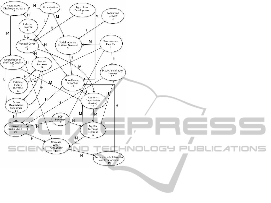
Figure 1: Fuzzy Cognitive map for M
´
exico city’s water
availability system.
3 ANALYSIS
3.1 Analysis of Feedback Processes,
Social and Climate Drivers
Our first analysis identified the feedback processes in
the map. The feedbacks are important because they
are the parts of the network that once they are ini-
tiated, the nodes constituting them will continue in-
teracting, even though the drivers are turned off. We
identified four feedbacks in the map:
• The first one is between the nodes 12 and 14, and it
represents the process between erosion increase and
the basins degradation (in the Cutzamala). A simi-
lar structure is between nodes Aquifers degradation
(Basins, 15) and Aquifer recharge decrease (17).
• The third process is constituted by nodes 13 (non
planned extraction), 15 (aquifers degradation basins),
17 (aquifer recharge decrease), 18 (decrease in water
availability), and 19 ( social and administrative con-
flicts increase).
• The fourth one is among concepts 13, 16, 18, 19,
and 13.
When any node in a feedback is activated, the pres-
ence of the signal remains in the map, and only dis-
appear if it is damped by fractionary weights at the
edges.
We analyzed the map using the technique of the
adjacent matrix and the vector state described section
1. We iterate using equation 1. We will denote de t-th
iteration by v
t
In order to check the feedback processes we
started climate and social drivers separately. In the
first case, starting climate drivers i.e. Temperature
increase and PCP decrease (the initial vector had a 1
in its first and second entrances), without considering
in this case extreme events, the system reached the
final vector in five iterations:
v
5
= [ 0 0 0 0 0 0 0 0 0 0 0 0 1 0 1 1 1 1 1 0 ]
Which means that together the increase of tem-
perature and the PCP decrease, will trigger nodes
13 (non-planned extraction), 15 (aquifers degrada-
tion, basins), 16 (decrease in dams levels), 17 (aquifer
recharge decrease), 18 (decrease of water availabil-
ity), and 19 (social and administrative conflicts in-
crease).
When nodes 3 (population growth), 4 (agriculture
development), 5 (urbanization), and 6 (industry
growth) were activated, the system converged in five
iterations to the vector:
v
5
= [ 0 0 0 0 0 0 0 0 0 0 0 1 1 1 1 1 1 1 1 0 ]
Which differs from our last result only by the
nodes 12 (erosion increase) and 14 (basins degrada-
tion, Cutzamala). When we considered C
1
→ C
11
the
resulting vectors were equals.
In both cases, we turned on the forcers only in the
initial vector (v
0
) and we let the system evolve. As
expected, the nodes with feedback remained ON even
though the driver was turned OFF.
We observed that the resulting vectors, forcing cli-
mate or social nodes, differ only by two nodes. This
indicates that nodes 13 (non-planned extraction), 15
(aquifers degradation basins), 16 (decrease in dams
levels), 17 (aquifer recharge decrease), 18 (decrease
of water availability), and 19 (social and administra-
tive conflicts increase) are driven by climate and so-
cial factors.
3.2 Hidden Patterns
Once we identified the feedback processes, we ana-
lyzed the map in the cases where we kept the forcing
after each iteration. These cases showed the final
states, when the forcer remained in the system. For
this analysis we considered the state vector and the
AFuzzyCognitiveMapforMéxicoCity'sWaterAvailabilitySystem
497

adjacent matrix with values in the set {0, 1}. Forcing
the system to different configurations showed how
the system responds to various initial conditions. We
used the three following configurations:
a. First we turned ON the Temperature increase and
PCP decrease and turned OFF the concepts 3, 4,
5 and 6. This showed how the system responds to
persistent climate forcing.
b. Turned OFF the Temperature increase and the
PCP decrease, and turned ON the concepts 3, 4, 5
and 6. Which considers only the social forcing of the
system.
c. We turned the Temperature increase and PCP
decrease ON, as well as concepts 3, 4, 5, and 6.
Which showed the system’s behavior having both
climate and social forcing.
In the first case (a), turning ON the nodes 1 and 2
(Temperature increase and PCP decrease), the system
converged in three iterations to the vector:
v
3
= [ 1 1 0 0 0 0 0 0 1 0 0 0 1 0 1 1 1 1 1 1 ]
This last result means that keeping nodes 1 and 2
forced increases the concepts: water social demand,
non-planned extraction, aquifers degradation (in
basins), decrease in dams levels, aquifer recharge
decrease, decrease in water availability, and social
and economic conflicts.
When node 11 was turned ON (extreme events
increase) together with nodes 1 and 2, the system
converged in three iterations to:
v
3
= [ 1 1 0 0 0 0 0 0 1 0 1 1 1 1 1 1 1 1 1 1 ]
With this configuration, nodes 12 (erosion in-
crease), and 14 (basin degradation, Cutzamala) were
turned ON.
In the case (b), when we turned OFF the nodes 1,
2, and 11, but instead we turned ON the nodes 3, 4, 5,
and 6, the system converged in four iterations to:
v
4
= [ 0 0 1 1 1 1 1 1 1 1 0 1 1 1 1 1 1 1 1 0 ]
Nodes 7 (waste waters discharge increase), 8
(vegetal cover loss), were turned ON and node 10
(degradation in water quality), and node 20 (evapo-
transpiration increase) were turned OFF.
Case (c), we turned ON the concepts 1, 2, 3, 4, 5,
6, and 11. The system converged in three iterations to
the vector:
v
3
= [ 1 1 1 1 1 1 1 1 1 1 1 1 1 1 1 1 1 1 1 1 ]
The difference between only considering temper-
ature increase (1) and PCP decrease (2) in compari-
son of turning ON the nodes population growth (3),
agriculture development (4), urbanization (5), and in-
dustry growth (6), both keeping the forcer, are basi-
cally the nodes: waste waters discharge increase (7),
vegetal cover loss (8), degradation in the water qual-
ity (10), erosion increase (12) and basins degradation,
Cutzamala (14). Notice that this nodes were turned
on when social forcers were ON.
3.3 Considering Climate Predictions of
Models
Although the climate drivers on M
´
exico city do not
completely depend on the processes developed there
(over the city), we know how they change and in-
teract by following the predictions given by the cli-
mate models (Oglesby et al. 2010). Different pre-
dictions allowed us to use the model we created to
explore different scenarios. The climate forcers in the
model are: temperature increase, PCP decrease, and
extreme events increase. The relations among these
three concepts, considering the scenarios of precipita-
tion decrease, and its opposite, precipitation increase,
are shown in the next image (Figure 2).
Figure 2: Interaction among climate forcers considering the
scenarios of precipitation decrease and increase.
As we said, the scenarios stated by the models
suggest different relations between the nodes tem-
perature increase and PCP decrease. Some models
suggest that if the temperature increases, the amount
of precipitation will decrease, while other models
suggest the opposite (Oglesby et al 2010). So, in the
map we considered positive and negative causality
separately for different scenarios. On the other hand,
all the models predicted an increase in extreme
events, but they ranged in their predictions among
intensity and frequency of the events. So the edge
from temperature increase to extreme events increase
is considered to be positive. If we assume that an
SIMULTECH2013-3rdInternationalConferenceonSimulationandModelingMethodologies,Technologiesand
Applications
498

increase in temperature causes an increase in the
PCP decrease and an increase in extreme events,
and running the model with these characteristics, i.e.
connecting node 1 with nodes 2 and 11, and restarting
node 1 after each iteration we have in four iterations
the following vector:
v
∗
4
= [ 1 1 0 0 0 0 0 0 1 0 1 1 1 1 1 1 1 1 1 1]
Which in comparison with the vector v
3
obtained
in the case (a) in section 3.2, when nodes 1 and 2
were forced, differs in nodes 11, 12 and 14.
v
3
= [ 1 1 0 0 0 0 0 0 1 0 0 0 1 0 1 1 1 1 1 1 ]
Considering that an increase in temperature
causes a decrease in PCP decrease (i.e. an increase in
PCP), in five iterations we have:
v
5
= [1 -1 0 0 0 0 0 0 1 0 1 1 1 1 1 1 1 1 1 1]
As seen, the only difference with respect to v
∗
4
is
the −1 in the node 2. Which means that even though
we considered an increase in PCP, the structured
interactions in the map have kept the tendency. This
is due to the fact that many nodes have more than one
node which is activating them, therefore, the sum of
the interactions is more than one, before the threshold
function.
With our approach of 0 and 1 for edges and values,
this is as far as we can go. But is very intuitive that
different processes have different amounts of causal-
ity, e.g. we know that temperature increase causes
social water demand increase, as well as evapotran-
spiration increase, but the strength of causality could
be different. It is convenient at this point to assign
pondered weights for each process in the map.
It is important to emphasize that we are evaluating
the map in a qualitative way, and assigning weighted
values only indicates a degree of causality among
concepts. We are not assuring, by indicating 0.5 for
a specific edge, that one concept causes exactly 0.5
the other. But, pondering the edges we gain intuition
about the map’s importance and sensitivity to each
process. These weighted values can be assigned by
expert’s opinion or proposed assuming specific con-
ditions we want to analyze.
3.4 Considering weighted Edges for
Sensitivity Analysis
In the previous analysis, we only considered positive
or negative causality in order to figure out the gen-
eral behavior of the system. However, this assump-
tion requires each edge to be either positive or neg-
ative, but with the same causality value. Neverthe-
less, we know that different processes have different
amounts of causality, for example, it could be intu-
itive that the temperature increase will have different
impacts in social water demand increase and in evapo-
ration increase, and this is an interesting thing to ana-
lyze. As the next example will show, these changes in
the value of interactions will lead different final states
for different edges values. Then, when we consider
weighted edges, the map’s behavior is qualitatively
different. In this case, some processes occur slowly
and some times their values will stabilize in a differ-
ent point.
For example, the following vector shows the state vec-
tor resulting from considering a value of 0.5 for each
edge after 10 iterations, when the system converges
into an equilibrium state given by:
v
10
= [ 1 0.5 0 0 0 0 0 0 0.5 0 0.5 0.33 0.44 0.16
0.61 0.80 0.80 0.79 0.39 0.5]
We can see how different nodes reached different
values in a new equilibrium state of the system. As
we said, we have considered all edges with value of
0.5 and we have restarted v[1] = 1 after each iteration.
In the Figure 3, the upper graph shows the evolution
of the concepts: erosion increase(12), non-planned
extraction (13), basins degradation (Cutzamala) (14),
aquifers degradation (basins) (15), decrease in dams
levels (16), aquifer recharge decrease (17), decrease
water availability (18), and social and administrative
conflicts increase (19). Concepts 3, 4, 5, 6, and 7
(which correspond with social forcers) were turned
off. Concepts 8 and 10 were not activated, because
they depend on the social forcers. Finally, the value
of C
1
(1), remained equal to 1, and the concepts 2, 9,
11 and 20 were not shown, because as they are only
activated by the concept C
1
, they remained with value
of 0.5. When upper and bottom graphs are compared,
it can be observed how dependent is the final value
of the concepts with the value of the edges. In the left
graph we used the same configuration but we changed
the sign in the edge C
1
→ C
2
which is taken as −0.5.
In this case the state vector after 10 iterations is:
v
10
= [ 1 -0.5 0 0 0 0 0 0 0.5 0 0.5 0.33 0.28 0.16
0.18 0.22 0.09 0.15 0.07 0.5]
These results show that the model is highly sen-
sible to changes in the edge values, sings, and initial
conditions, however we can see that the concept’s val-
ues tendency to growth remains.
AFuzzyCognitiveMapforMéxicoCity'sWaterAvailabilitySystem
499
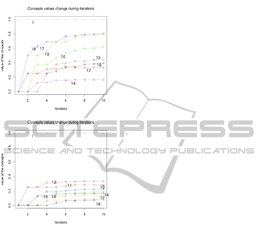
Figure 3: Upper graph: evolution of the concepts erosion
increase(12), non-planned extraction (13), basins degrada-
tion (Cutzamala) (14), aquifers degradation (basins) (15),
decrease in dams levels (16), aquifer recharge decrease (17),
decrease water availability (18), and social and administra-
tive conflicts increase (19) after 10 iterations with all the
edges having a value of 0.5. Bottom: the same configura-
tion, but changing edge C
1
→ C
2
which is taken as −0.5. In
both graphs concept C
1
is in pink color.
3.5 Using weighted Edges
As we just discussed, the behavior of the model is
completely different depending on the value of the
edges. Nevertheless, sometimes is difficult to ponder
processes of different nature, like the increase in so-
cial and administrative conflicts and the temperature
increase. For this reason, this process involves the
experts opinion. We assigned the value of the edges
by consulting Dr. Escolero. We asked him to assign
“how much one node causes another” using linguistic
quantities. In this case, we chose as linguistic quan-
tities: low (L), medium (M), and high (H). These lin-
guistic values are shown in Figure 1.
This map contains the expert opinion, which is
based on the knowledge of the system. Now, in order
to analyze it using the technique of the adjacent ma-
trix and the vector sate, we divided the interval [0,1]
in three subsets, each one of them representing one
set of strength of causality. Then, we chose a rep-
resentative value for each set which was used as its
corresponding entrance in the matrix. In this case we
chose the values of 0.3 for low, 0.6 for medium, and
0.9 for high. And we selected medium causality for
the edge C
1
→ C
2
and low for C
1
→ C
11
.
Then, we ran the model using these values,
starting only C
1
with value of 1 and keeping the
forcing. The state vector after six iterations is:
v
6
= [1 0.9 0 0 0 0 0 0 0.6 0 0.3 0.16 1 0.08 1 1 1
1 0.9 0.9]
Concepts 2 (0.9 PCP decrease), 9 (0.6 social in-
crease in water demand), 11 (0.3 extreme event in-
crease), and 20 (0.9 evapotranspiration increase) re-
mained constant, as they were activated by C
1
. Con-
cepts 3, 4, 5, and 6 (social forcers) were not acti-
vated. Concepts 7, 8, and 10 depended on the so-
cial forcers. In figure 6, we represented concepts ero-
sion increase(12), non-planned extraction (13), basins
degradation (Cutzamala) (14), aquifers degradation
(Basins) (15), decrease in dams levels (16), aquifer
recharge decrease (17), decrease water availability
(18), and social and administrative conflicts increase
(19) after 6 iterations.
In Figure 4 Upper, concepts 12 (erosion increase)
and 14 (basins degradation, Cutzamala), which form a
feedback cycle, stabilize at 0.16 and 0.08 respectively,
as well as concept 19 social and administrative con-
flicts increase with a value of 0.9. All other concepts
exceeded the value of one, and thus they were lim-
ited to one. These are 13 (non-planned extraction), 15
(aquifers degradation (basins)), 16 (decrease in dams
levels), 17 (aquifer recharge decrease), and finally 18
(decrease water availability) which is superposed with
concept 13.
With the same map, we started and kept the
social drivers 3 (population growth), 4 (agriculture
development), 5 (urbanization), and 6 (industry
growth) forced, and turned off C
1
(Figure 4 Bottom).
After six iterations we obtained:
v
6
= [0 0 1 1 1 1 1 1 1 0.6 0 1 1 0.78 1 1 0.6 1 0.9
0]
Concepts that depend of C
1
remained off. Con-
SIMULTECH2013-3rdInternationalConferenceonSimulationandModelingMethodologies,Technologiesand
Applications
500
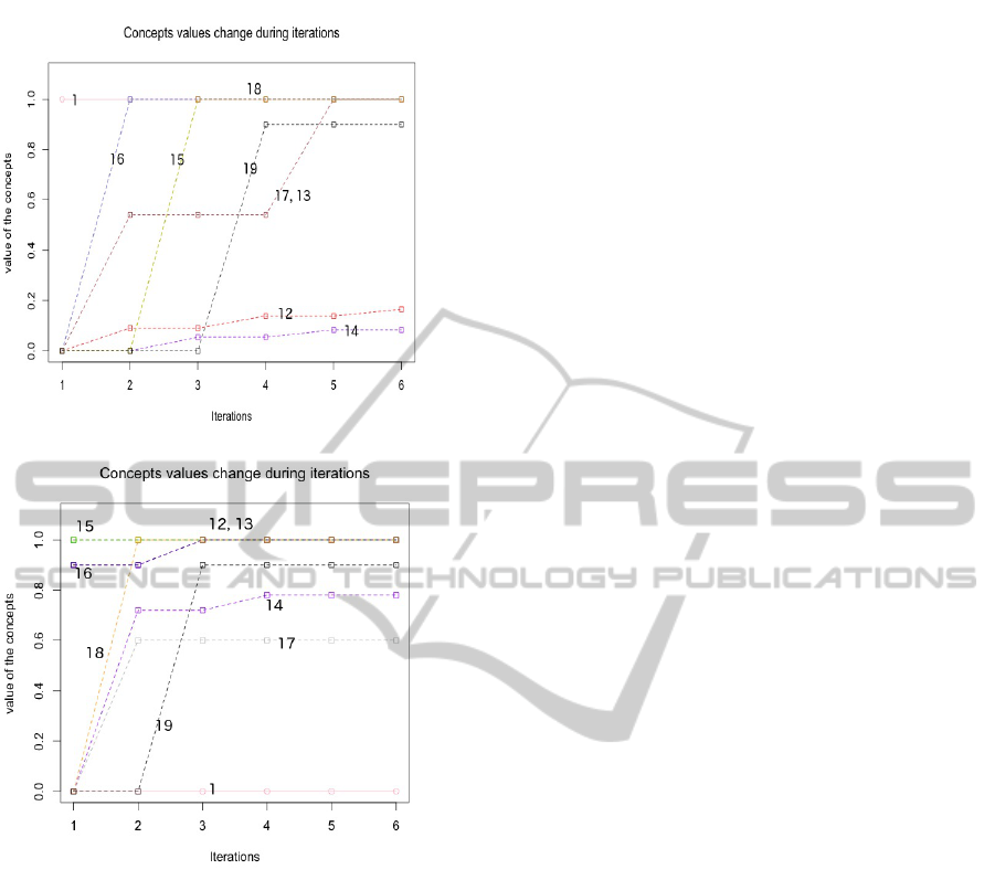
Figure 4: Upper: Evolution of the concepts erosion in-
crease(12), non-planned extraction (13), basins degradation
(Cutzamala) (14), aquifers degradation (basins) (15), de-
crease in dams levels (16), aquifer recharge decrease (17),
decrease water availability (18), and social and administra-
tive conflicts increase (19) after 6 iterations. Keeping forced
C
1
denoted as 1. Bottom: Evolution of the concepts 12, 13,
14, 15, 16, 17, 18 and 19. Turning on the social forcers 3,
4, 5, and 6, and turning off C
1
.
cepts 7, 8 and 9, which depend directly of activated
concepts, went to one at the first iterations. Con-
cept 10 was activated constantly by Concept 7. Con-
cept 11 remained off. Concepts 12 (erosion increase)
and 13 (non-planned extraction) went to one. Con-
cept 14 (basins degradation Cutzamala) stabilized at
0.78. Concepts 15 (aquifers degradation (Basins))
and 16 (decrease in dams levels) went quickly to 1.
Concept 17 (aquifer recharge decrease) stabilized in
0.6. While Concept 18 (decrease in water availabil-
ity) went to 1 after 3 iterations. And finally, Con-
cept 19 (social and administrative conflicts increase)
remained as 0.9 because it is activated by Concept 18.
The substantial difference between forcing the sys-
tem with social or climatic factors is shown in nodes
12 (erosion Increase) and in 14 (basins degradation,
Cutzamala).
3.6 Min - Max Criteria for the Analysis
of Influences over the Decrease in
Water Availability
As we said in the introduction, we can use the
min - max criteria to analyze how much a node
causes another. In this case, we wanted to compare
the influence of climatic and social factors over
the decrease in water availability. To estimate the
total effect of temperature increase over decrease in
water availability, we had to consider the effective
paths: I
1
(1, 9, 13, 16, 18) = min{M, H, H, H, H} = M,
I
2
(1, 9, 13, 15, 17, 18) = min{M, H, H, M, M} =
M, I
3
(1, 20, 16, 18) = min{H, H, H} = H,
I
4
(1, 20, 17, 18) = min{H, H, M} = M,
I
5
(1, 2, 16, 18) = min{M, H, H} = M,
I
6
(1, 2, 17, 18) = min{M, H, H} = M,
I
7
(1, 11, 12, 14, 16, 18) = min{L, H, M, H, H} = L.
The total effect is the maximum of the indirect
effects, in this case equal to H. But if we analyze
closely the only path which has indirect effect H is
I
3
(1, 20, 16, 18) = min{H, H, H} = H, so if we want
to change the effect of the temperature increase over
decrease in water availability we need to focus on
the processes among: temperature increase → evap-
oration increase. evaporation increase → decrease
in dams levels. decrease in dams levels → decrease
water availability. These three edges are practically
out of our control, but we can infer that if we want to
counteract the influence of temperature increase over
the system, we must probably focus on strategies to
avoid the decrease in dam levels.
On the other hand, when we analyzed the so-
cial drivers (as a whole), we found that the total
effect of all of them is High, but only one Indi-
rect effect which is ”High” is I
3→18
(3, 9, 13, 16, 18) =
min{H, H, H, H}. Like we just discussed, this obser-
vation can also help us for decision making and strate-
gic planning.
4 CONCLUSIONS
We could observe, from the feedback processes form
section 3.1, that both social and climatic drivers will
lead the system to an undesirable state. The only dif-
ference between the two feedbacks of social and cli-
AFuzzyCognitiveMapforMéxicoCity'sWaterAvailabilitySystem
501

matic drivers are nodes 12 (erosion increase) and 14
(basins degradation, Cutzamala). Both of them are
turned on due to social drivers.
The results found in section 3.2 reconfirm that so-
cial drivers have a high influence over the network.
By analyzing the hidden patterns obtained by keep-
ing the different drivers ON, the difference were in
the following nodes: waste waters discharge increase
(7), vegetal cover loss (8), degradation in the water
quality (10), erosion increase (12) and basins degra-
dation, Cutzamala (14). That were activated by the
social drivers and not by the climatic drivers.
In section 3.3 the system was forced under two
different climate change scenarios. The considera-
tions made were the decrease and the increase in PCP.
The resulting vector in comparison with the vector v
3
obtained in the case (a) in section 3.2,(base scenario,
that we obtained when nodes 1 and 2 were forced in
section 3.2), differed only on the nodes 11, 12 and
14, and there was no difference when we considered
a PCP decrease or increase. This is a consequence of
the particular structure of the system.
When considering weighted edges for the whole
system (section 3.5) we validated the results obtained
in previous sections. Since the difference between
social and climatic factors was in nodes 12 (erosion
increase) and in 14 (basins degradation, Cuzamala)
once again. In section 3.4 we could identify that, even
though the system behavior was sensible to changes in
the weights, it maintained the general tendency.
In section 3.6 we found that the “causality” that
climate and social drivers (as a whole) imparted over
the decrease in water availability was ”high”. But in
both cases the “high” causality is centered on a par-
ticular processes.
From these results we can conclude, first of all,
that the system is significantly affected by climatic an
social drivers, i.e. both can trigger the system and lead
it into an undesirable state. Moreover, it appears that
the strength of social drivers are greater than those of
the climatic drivers. Since the social drivers in Mex-
ico city are currently on, climatic drivers will act as an
accelerator for the degradation processes on the water
system. Therefore both drivers should be taken into
account for policies design.
The general recommendations after the analysis
are focused on two branches:
Climatic drivers:
I
1→18
(1, 20, 16, 18) = min{H, H, H} = H.
Social drivers:
I
3→18
(3, 9, 13, 16, 18) = min{H, H, H, H}.
Which have a “high” influence over water availabil-
ity. Further investigation is needed for each node and
edge on the two branches, to design policies and so-
lutions.
A general conclusion based on this FCM for wa-
ter availability in Mexico city, is that the degradation
process will occur, given the present conditions, with
climatic drivers or without them, as social drivers are
more influential on the network. The social situation
that operates over the water system is pushing the sys-
tem into an undesirable state, and only with a more in
depth study of the interactions among the nodes we
will know whether or not the system can return to its
equilibrium state.
It is remarkable that the system’s dynamic did not
change wether a consideration of an increase or a de-
crease in precipitation was made. It is also notable
how the system is sensible to changes in the weight of
the edges but without changing its general tendency.
ACKNOWLEDGEMENTS
The present work was developed with the support of
the Programa de Investigaci
´
on en Cambio Clim
´
atico
(PINCC) of the Universidad Nacional Aut
´
onoma de
M
´
exico (UNAM).
REFERENCES
Cakmak E, Dudu H, Eruygur O, Ger M, Onurlu S, and
Tongu
¨
O. Participatory fuzzy cognitive mapping
analysis to evaluate the future of water in the Sey-
han Basin. Journal of Water and Climate Change In
Press, Uncorrected Proof IWA Publishing 2013 —
doi:10.2166/wcc.2013.029
Elpiniki P, and Areti K (2012). Using Fuzzy Cognitive
Mapping in Environmental Decision Making and
Management: A Methodological Primer and an
Application, International Perspectives on Global
Environmental Change, Dr. Stephen Young (Ed.),
ISBN: 978-953-307-815-1, InTech, Available from:
http://www.intechopen.com/books/international-
perspectives-on-global-environmental-change/using-
fuzzy- cognitive-mapping-in-environmental-decision-
making-and-management-a-methodological-prime
Escolero, F. (2009). Vulnerabilidad de las fuentes
de abastecimiento de agua potable de la Ciudad
de M
´
exico en el contexto de cambio clim
´
atico.
(“Vulnerability of fresh water sources in M
´
exico
city in the context of climate change”) Available
online at http://www.cvcccm-atmosfera.unam.mx/
documents/investigaciones/pdf/Agua Escolero %20In
fFinal org.pdf Accessed March 2013.
IPCC (2007) Climate Change 2007: The Physical Sci-
ence Basis. Contribution of Working Group I to the
Fourth Assessment Report of the Intergovernmental
Panel on Climate Change [Solomon, S., D. Qin, M.
Manning, Z. Chen, M. Marquis, K.B. Averyt, M. Tig-
nor and H.L. Miller (eds.)]. Cambridge University
SIMULTECH2013-3rdInternationalConferenceonSimulationandModelingMethodologies,Technologiesand
Applications
502

Press, Cambridge, United Kingdom and New York,
NY, USA, 996 pp.
Kosko, B. (1988). Fuzzy Cognitive Maps. International
Journal of Man-Machine Studies. 24, 65-75.
Kosko, B. (1992). Neural Networks and Fuzzy Systems,
Prentice Hall, NJ.
Nguyen, H. Prasad, N. Walker, C. Walker, E. 2003. A
First Course in Fuzzy and Neural Control. Chapman
& Hall/CRC. USA, 296 pp.
Oglesby, R. Rowe, C. and Hays, C. (2010). Cli-
mate Impacts in Mesoamerican Countries: Re-
sults from Global and Regional Climate Mod-
els. University of Nebraska-Lincoln. Available on-
line at: http://weather.unl.edu/RCM/reports/impacts/
Mesoamerica Climate Impacts.pdf Accessed April
2013.
Pelez, E. Bowles, J. (1996). Using Fuzzy Cognitive Maps as
a System Model for Failure Modes and Effects Anal-
ysis Information Sciences 88, 177-199.
Soler L, Kok K, Camara G, and Veldkamp A. Using fuzzy
cognitive maps to describe current system dynamics
and develop land cover scenarios: a case study in the
Brazilian Amazon. Journal of Land Use Science i
First, 2011, 127.
Stylios, C.D. Georgopoulos, V.C. ; Groumpos, Peter P. In-
troducing the theory of fuzzy cognitive maps in dis-
tributed systems. Proceedings of the 1997 IEEE In-
ternational Symposium on Intelligent Control, 1997.
Stylios C.D. and Groumpos P.P, “Modeling Complex Sys-
tems Using Fuzzy Cognitive Maps, IEEE Transac-
tions on Systems, Man and Cybernetics: Part A Sys-
tems and Humans. (IF:0,555) Vol. 34, No 1 pp. 155-
162 (2004).
Zadeh, L. (1965). Fuzzy Sets. Information and Control. 8,
338-353.
AFuzzyCognitiveMapforMéxicoCity'sWaterAvailabilitySystem
503
