Tyre Footprint Reconstruction in the Vehicle Axle Weight-in-Motion

Measurement by Fibre-optic Sensors

Alexander Grakovski, Alexey Pilipovecs, Igor Kabashkin and Elmars Petersons

Transport and Telecommunication Institute, 1 Lomonosova Street, Riga, Latvia

Keywords: Transport Telematics, Weigh-in-Motion, Fibre-optic Sensor, Tyre Footprint.

Abstract: The problem of measuring road vehicle’s weight-in-motion (WIM) is important for overload enforcement,

road maintenance planning and cargo fleet managing, control of the legal use of the transport infrastructure,

road surface protection from the early destruction and for the safety on the roads. The fibre-optic sensors

(FOS) functionality is based on the changes in the parameters of the optical signal due to the deformation of

the optical fibre under the weight of the crossing vehicle. A fibre-optic sensor responds to the deformation,

therefore for WIM measurements it is necessary to estimate the impact area of a wheel on the working

surface of the sensor called tyre footprint. This information is used further for the estimation of the vehicle

wheel or axle weight while in motion. Recorded signals from a truck passing over a group of FOS with

various speeds and known weight are used as an input data. The results of the several laboratory and field

experiments with FOS, e.g. load characteristics according to the temperature, contact surface width and

loading speed impact, are provided here. The examples of the estimation of a truck tyre surface footprint

using FOS signals are discussed in this article.

1 INTRODUCTION

The worldwide problems and costs associated with

the road vehicles overloaded axles are being tackled

with the introduction of the new weigh-in-motion

(WIM) technologies. WIM offers a fast and accurate

measurement of the actual weights of the trucks

when entering and leaving the road infrastructure

facilities. Unlike the static weighbridges, WIM

systems are capable of measuring vehicles traveling

at a reduced or normal traffic speeds and do not

require the vehicle to come to a stop. This makes the

weighing process more efficient, and in the case of

the commercial vehicle allows the trucks under the

weight limit to bypass the enforcement.

There are four major types of sensors that have

been used today for a number of applications

comprising the traffic data collection and overloaded

truck enforcement: piezoelectric sensors, bending

plates, load cells and fibre-optic sensors (McCall et

al., 1997); (Teral, 1998). The fibre-optic sensors

(FOS), whose working principle is based on the

change of the optical signal parameters due to the

optic fibre deformation under the weight of the

crossing road vehicle (Batenko et al., 2011); (Malla

et al., 2008), have gained popularity in the last

decade.

Analysis of the WIM current trends indicates that

optical sensors are more reliable and durable in

comparison to the strain gauge and piezoelectric

sensors. Currently the two FOS types based on two

main principles are used:

 Bragg grating (the change of diffraction in a

channel under deformations);

 The fibre optical properties (transparency,

frequency, phase and polarization) change during

the deformations.

A lot of recent investigations are devoted to the

peculiarities of the construction and applications of

the sensors, using different physical properties. The

data presented in this publication have been received

using SENSOR LINE PUR experimental sensors

(SENSORLINE, 2010) based on the change of the

transparency (the intensity of the light signal) during

the deformation.

527

Grakovski A., Pilipovecs A., Kabashkin I. and Petersons E. (2013).

Tyre Footprint Reconstruction in the Vehicle Axle Weight-in-Motion Measurement by Fibre-optic Sensors.

In Proceedings of the 10th International Conference on Informatics in Control, Automation and Robotics, pages 527-536

DOI: 10.5220/0004620905270536

 SciTePress

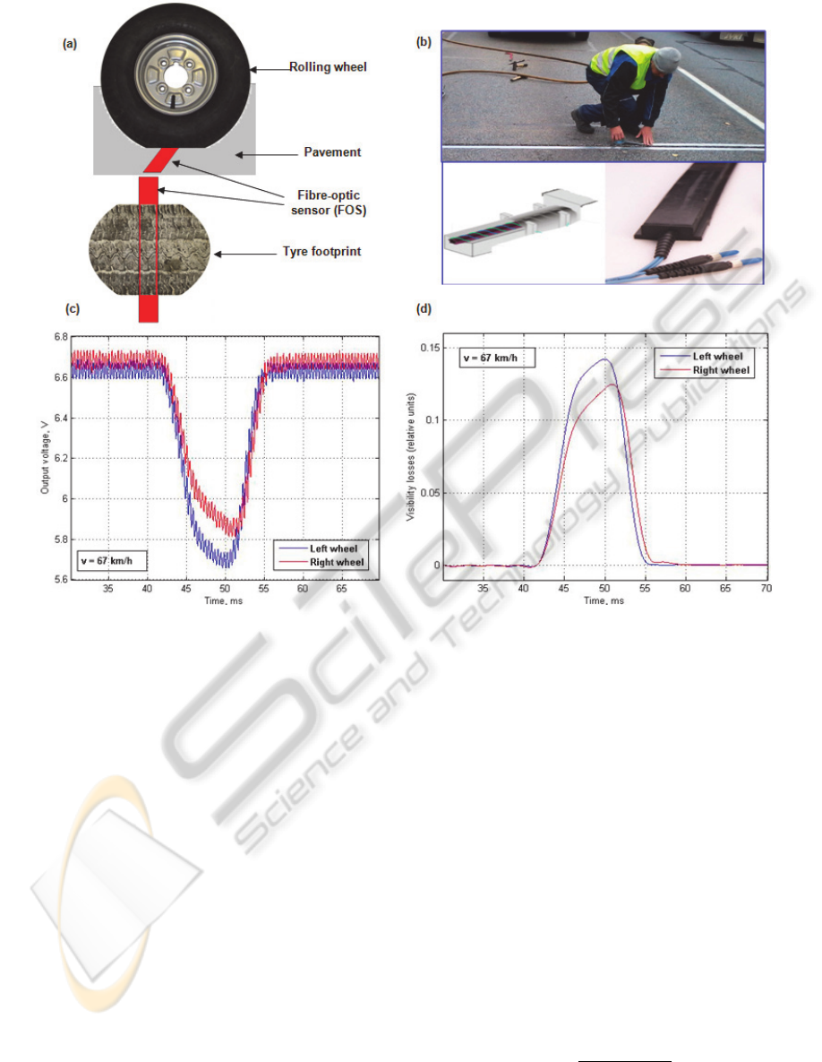
Figure 1: (a) Fibre optic sensor’s position against the wheel and tyre footprint, (b) SENSORLINE PUR installation and

construction of the sensor, (c) FOS output voltage, (d) Visibility losses as the function of pressure after pre-processing

(filtering).

2 AXLES

WEIGHING-IN-MOTION

PRINCIPLES

The fibre optic weight sensor is the cable consisting

of a photoconductive polymer fibres coated with a

thin light-reflective layer (Fig. 1(b)). A light

conductor is created in such a way that the light

cannot escape. If one directs a beam of light to one

end of the cable, it will come out from the other end

and in this case the cable can be twisted in any

manner. To measure the force acting on the cable,

the amplitude technology is more appropriated for

the measurements based on measuring of the optical

path intensity, which changes while pushing on the

light conductor along its points.

At these points the deflection of a light conductor

and reflective coating occurs, that is why the

conditions of light reflection inside are changed, and

some of it escapes. The greater the load the less light

comes from the second end of the light conductor.

Therefore the sensor has the unusual characteristic

for those, familiar with the strain gauges: the greater

the load the lower the output is. Apart from the fact

that it is reversed and in addition to this it is non-

linear.

In order to avoid the inaccuracy of zero load

level we need to exclude the high frequency

components from the voltage signal at the output of

the sensor’s transducer by filtering, as well as to

recalculate the voltage signal U(t) (Fig. 1(c)) into the

relative visibility losses signal V(t) (Fig. 1(d)),

directly related to the weight pressure on the FOS

surface. It can be done by the transformation (1):

tUU

)(





(1)

where U

is the voltage of sensor’s output with zero

ICINCO2013-10thInternationalConferenceonInformaticsinControl,AutomationandRobotics

528

Figure 2: Experimental truck “Volvo FH12” with full load 36900 kg.

Table 1: The reference static axle weights.

Date: 20.04.2012 (Air Temperature +12

С).

Reference axle weight (tons): 7.296 12.619 5.509 5.641 5.844

load. The signal transformation to the relative

visibility losses signal V(t) gives the possibility to

compare signals for different measurements in

different conditions.

Fibre optic load-measuring cables are placed in

the gap across the road, filled with resilient rubber

(Fig. 1(b)). The gap width is 30 mm. Since the

sensor width is smaller than the tyre footprint on the

surface, the sensor takes only part of the axle weight.

Two methods are used in the existing systems to

calculate the total weight of the axle [2, 3]: the

Basic Method and the Area Method. The following

formula is used to calculate the total weight of the

axis using the Basic Method:

ttha

PAW 

(2)

where W

– weight on half-axle, A

– area of the

tyre footprint, P

~ V(t) – air pressure inside the tyre

and, according to Newton’s 3

law, it is proportional

to the axle weight.

As we can see the exact values of the formula

factors are unknown. The area of the tyre footprint is

calculated roughly by the length of the output

voltage impulse, which, in its turn, depends on the

vehicle speed. The Area Method uses the

assumption that the area under the recorded impulse

curve line, in other words – the integral,

characterizes the load on the axle. To calculate the

integral, the curve line is approximated by the

trapezoid. In this case the smaller the integral – the

greater the load. This method does not require

knowing the tyre pressure, but it requires the time-

consuming on-site calibration. Also, it has to be kept

in mind that the time of the tyre crossing the sensor

is too small to get an electrical signal of high quality

for its further mathematical processing. We use the

Area method only for the tyre footprint area

definition in (2), but the pressure is measured from

the signal amplitude.

3 EXPERIMENTAL VEHICLE

PARAMETERS

There was the set of measurement experiments with

the roadside FOS sensors on April, 2012 in Riga,

Latvia. Loaded truck (Fig.2) was preliminary

weighed on the weighbridge with the accuracy <

1%.

Reference weights of the separate axles are given

in the Table 1. The output signals from FOS sensors

for truck speeds 70 km/h and 90 km/h are

demonstrated on Fig.3. It is evident that the signals

for the different speeds have been changing by

amplitude and the proportion of amplitudes does not

fit the axle weights (Fig.3). The reason of this

behaviour may be explained by FOS properties such

as weight (pressure) distribution along the sensor

length as well as sensor non-linearity and

temperature dependence.

4 FIBRE OPTIC SENSOR

PROPERTIES

Fibre-optic sensor (SENSORLINE PUR) output

light intensity changes due to the applied external

vertical force were measured using of the optical

interface SL MA-110 that was developed by

SensorLine GmbH (SensorLine, 2010). Laboratory

experiments with varying parameters (temperature,

steel plate width and load speed) were made at

Latvian University Institute of Polymer Mechanics

with electronically controlled compression machine.

TyreFootprintReconstructionintheVehicleAxleWeight-in-MotionMeasurementbyFibre-opticSensors

529

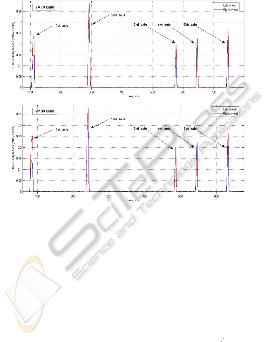
Figure 3: Examples of FOS signals of experimental truck for vehicle speeds 70 km/h and 90km/h respectively.

The first experiment examined the load

characteristic according to the temperature change:

FOS was placed into the tube of the soft thermal

insulation material in which chilled carbon dioxide

was circulating. The load from a compression

machine was applied to the sensor through the tube

and a 200 x 200 mm square steel plate (Figure 4(a)).

It was found during this experiment that the optical

response of the FOS was changing due to the

warming. And it is important to notice, that no

pressure was applied (Figure 4(b)).

FOS is permanently installed in the road surface,

therefore environment temperature changes affect

characteristics of the protective housing rubber

(stiffness) and the medium where the light

propagates. These changes introduce nonlinear

distortions which together with externally applied

pressure on a FOS are displayed at figure 4(c).

Relations between the load characteristics at the

different temperatures are displayed in the figure

4(d). These relations can be conditionally described

by polynomial approximation model:

),atata(LCLC

]C[]C[T 01

230



(3)

where LC

T[C]

is desired load characteristic at T

degrees, LC

30[C]

is load characteristic at 30

degrees and a

2,1,0

are coefficients of least square

optimisation calculated from figure 4(d).

In the real environment tyre footprint width may

vary depending on tyre size and inflation pressure,

which will result in the different force redistribution.

The second experiment shows this dependence

(figure 5(a)), these measurements were made at

constant temperature 14

C degrees and constant

loading speed 20 mm/s.

Relations between the load characteristics

obtained using the different steel plates are displayed

in figure 5(b). These relations can be conditionally

described by exponential approximation model:

),e(aLCLC

]mm[]mm[W

1200



(4)

where LC

W[mm]

is desired load characteristic with W

mm wide plate, LC

200[mm]

is load characteristic with

200 mm wide plate and a

1,2

are coefficients of least

ICINCO2013-10thInternationalConferenceonInformaticsinControl,AutomationandRobotics

530

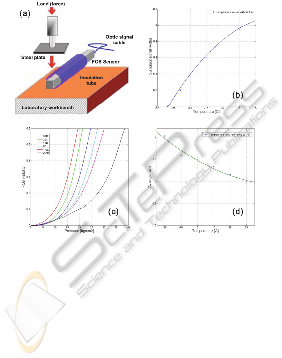
Figure 4: (a) Experimental laboratory equipment scheme, (b) FOS temperature dependence without applying load, (c) FOS

load characteristics at different temperatures and (d) Fitted model of FOS various temperature load characteristic ratio

values relative to 30

C degrees.

square optimisation calculated from figure 5(b).

The vehicles are crossing the FOS at the different

speeds and the sensor reaction is different due to its

inertia properties. Therefore the third experiment

was dedicated to study FOS output signal

dependence on applied force at the different speeds

(figure 6(a)): these measurements were made at the

constant temperature 17

C degrees and the steel

plate size 200 mm. Relations between the load

characteristics at the different applied speeds are

displayed in figure 6(b). These relations can be

conditionally described by power approximation

model:

),Sa(LCLC

]s/mm[.]s/mm[S

10660



(5)

where LC

X[mm/s]

is desired load characteristic at S

mm/s, LC

0.066[mm/s]

is load characteristic at 0.066

mm/s and a

1,0

are coefficients of least square

optimisation calculated from figure 6(b).

5 TYRE FOOTPRINT AND

WEIGHT ESTIMATION

As it is clearly seen from the expression (2), the At

area of the tyre footprint should be known to

calculate the axle weight by the registered FOS

signal (Batenko et al., 2011). The form of the signal

is non-symmetric and sufficiently distorted by the

rolling process of the wheel on the road surface (see

Figure 7(a)).

TyreFootprintReconstructionintheVehicleAxleWeight-in-MotionMeasurementbyFibre-opticSensors

531

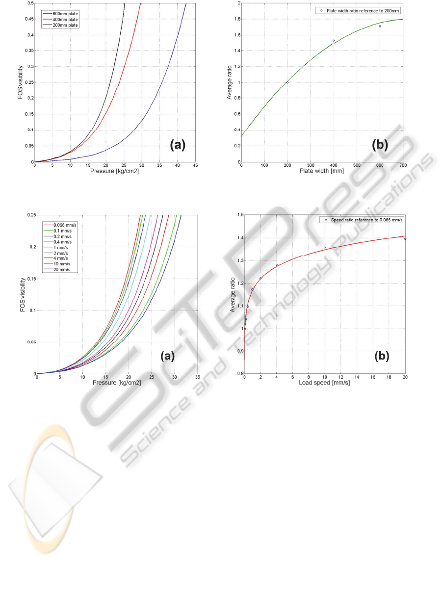
Figure 5: (a) FOS load characteristics with the different steel plate widths and (b) Fitted model of FOS various steel plate

width load characteristic ratio values relative to 200x200mm steel plate.

Figure 6: (a) FOS load characteristics at different load speeds and (b) Fitted model of FOS various load speed load

characteristic ratio values relative to 0.066 mm/s load speed.

One of the possible explanations of the signal

waveform distortion is the idea about the common

interaction of two factors (Krasnitsky, 2012):

vertical dead weight gravity of conditionally

immovable wheel (according to wheel geometry it

must be symmetric, see Figure 7(b)), and the force

of friction (it depends on the pavement and tyre

properties, wheel’s speed and weight, and its

expected waveform is asymmetric, see Figure 7(c)).

The problem of the decomposition of the non-

symmetric signal in two parts (symmetric and

asymmetric) can be solved by the polynomial

approximation using the least square method and the

further grouping of members with even and odd

powers separately or by standard even-odd

decomposition of the signal on finite window

(Mesco, 1984); (Vinay et al., 2006).

On the other hand, by assumption that the

vehicle moves uniformly and all forces maximally

compensate each other, we can accept that the

friction force is as minimal as possible (rolling

friction only without sliding friction). It is possible

to minimize the friction component magnitude

moving the axis of symmetry before the pulse (see

Figure 8(b)). It will be minimal at the position

conditionally named as the “mass centre” of the

pulse (see Figure 8(a)). The waveform of the friction

component on Figure 8(b)) sufficiently differs from

the same on Figure 7(c). Two maximums and two

minimums clearly locate the characteristic points for

the tire footprint estimation in the elliptic

approximation (see Figure 8(c)).

ICINCO2013-10thInternationalConferenceonInformaticsinControl,AutomationandRobotics

532

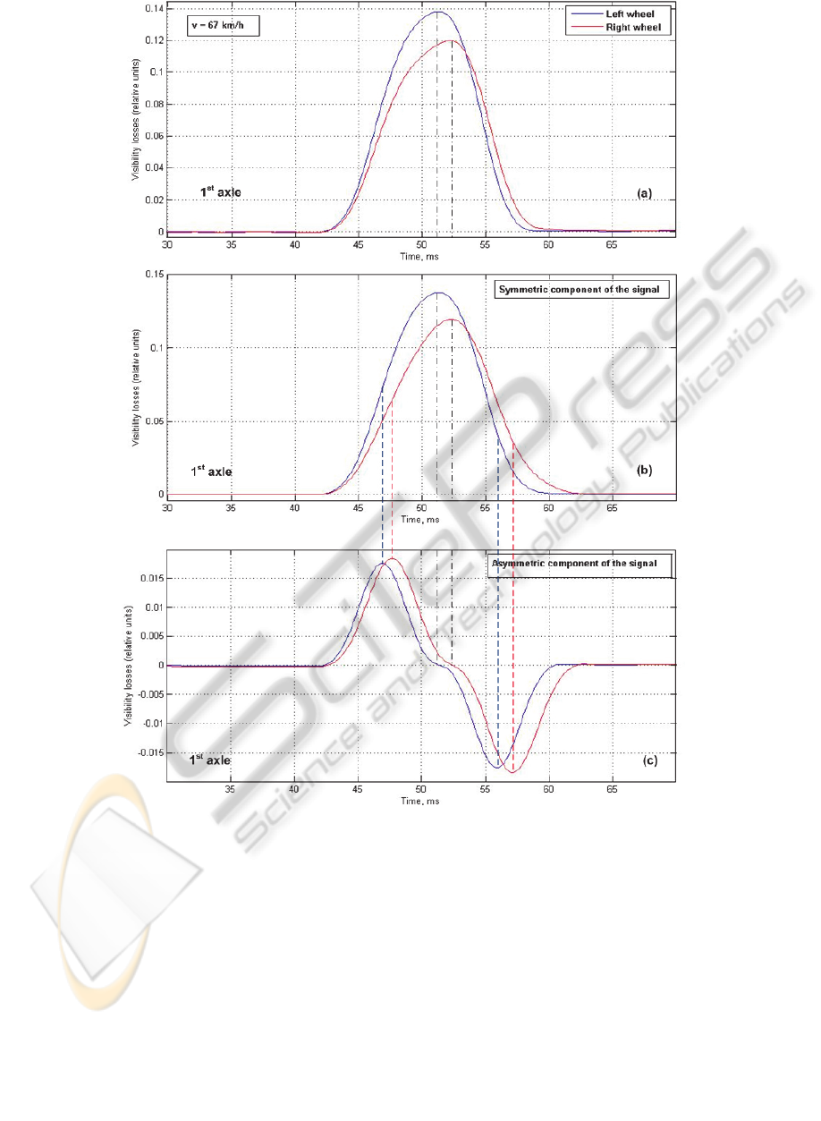
Figure 7: (a) FOS output signal in the form of visibility losses (formula 1), (b) Approximated vertical weight component

(symmetric), and (c) Approximated asymmetric component depending on horizontal velocity and friction (Krasnitsky, 2012).

Now the problem of the tyre footprint area

estimation may be solved. Multiplying the impulse

length by the speed of the wheel we can calculate

the length of the footprint. In the considered

examples (Figures 7 and 8) it is L

left

= 0.1905 m and

right

= 0.1976 m. It agrees with another data for the

wheel R22.5 and tyre width of 315 mm for the 1

axle. Full data of footprint lengths for experimental

cargo vehicle (see Figure 2 and Table 1) are the

following: left side wheels lengths are L

L12345

{0.1905 0.1652 0.1278 0.1354 0.1379}

meters, and right side wheels lengths are L

R12345

{0.1976 0.1799 0.1509 0.1449 0.1356} meters.

The difference between the lengths of each wheel

can be explained by the fact that the 2

axle has the

double-wheel, the trailer tyres but (axles No 3-5)

width is 385 mm.

Applying the sensors signal processing algorithm

together with the of estimation of the tyre footprint

area and approximation of the nonlinear

characteristics of the FOS (Figures 4, 5 and 6) for

the suitable range of temperatures, it is possible to

estimate the following weights of axles (Table 2).

TyreFootprintReconstructionintheVehicleAxleWeight-in-MotionMeasurementbyFibre-opticSensors

533

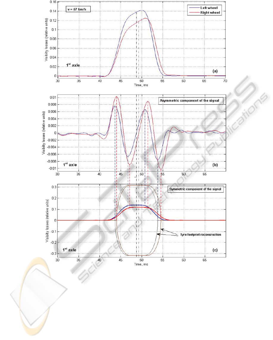
Figure 8: (a) FOS output signal in the form of visibility losses in dimensionless units, (b) Approximated vertical weight

component (symmetric), (c) Approximated asymmetric component and tire footprint reconstruction in case of minimal

friction condition.

As it can be seen from the Table 2, the most

preferred for the measurements are the velocity

ranges from 50 km/h and above: the measurement

errors of the axle loads do not exceed 10%, which is

consistent with the problem of the pre-selection of

the overloaded vehicles. The dynamics of vehicle

breaking or acceleration is more visible at the low

velocities. It can seriously distort the waveform of

asymmetric friction component and change

characteristic points for tyre footprint estimation.

The source of the relatively big measurement errors

at the low velocities are the distortion and footprint

area reconstruction errors because of the vertical

oscillations of the dynamic motion of the vehicle,

whose amplitudes are smaller at the higher speeds.

Taking into account the properties of each

individual sensor, the calibration of FOS should be

conducted twice: at first in the laboratory (load

characteristics in the temperature range from -20

to +30

C), and, secondly, after installing the sensor

in the road surface using the vehicles with allowed

but known weight.

ICINCO2013-10thInternationalConferenceonInformaticsinControl,AutomationandRobotics

534

Table 2: The results of the axle weight estimation and errors for the different measurements at the speeds 10-90 km/h (2-6

sets of measurements per speed bin).

Date: 20.04.2012 (Air Temperature +12

С)

Parameter: 1

axle 2nd axle 3rd axle 4th axle 5th axle

Reference axle’s weight (tons): 7.296 12.619 5.509 5.641 5.844

Group of speed: 10 km/h

1 Error for v=16 km/h 0.589% 0.855% -12.994% -10.317% -0.453%

2 Error for v=13 km/h -1.058% 10.985% -16.472% -8.316% 12.152%

Group of speed: 20 km/h

1 Error for v=19 km/h -2.176% 2.496% -3.417% 10.885% 11.251%

2 Error for v=20 km/h -0.046% 7.408% -18.445% -14.253% -3.248%

3 Error for v=17 km/h 0.104% 11.259% -24.200% -14.172% -9.916%

Group of speed: 50 km/h

1 Error for v=53 km/h 3.921% -4.982% -2.327% -3.582% -5.029%

2 Error for v=53 km/h 2.042% -1.114% -7.144% -4.676% -3.918%

3 Error for v=56 km/h -0.960% 0.278% -9.221% -0.203% -5.632%

4 Error for v=53 km/h 4.276% -0.762% -2.402% -1.905% -1.903%

5 Error for v=52 km/h -1.729% 1.864% -8.976% 2.880% -2.962%

Group of speed: 70 km/h

1 Error for v=73 km/h 2.969% -3.487% -4.746% 0.482% -2.497%

2 Error for v=74 km/h 2.455% -1.204% -4.474% 1.747% 0.183%

3 Error for v=72 km/h 4.699% -2.881% -1.259% -3.693% -1.093%

4 Error for v=74 km/h 4.879% -0.886% -0.923% 3.921% 1.865%

5 Error for v=75 km/h 4.314% -2.824% 3.493 1.918% 1.247%

6 Error for v=67 km/h -2.708% 2.749% 0.281% 4.664% 3.249%

Group of speed: 90 km/h

1 Error for v=86 km/h 0.499% 1.702% -8.152% -4.744% -3.859%

2 Error for v=85 km/h 4.149% -4.338% -5.907% 0.278% 0.094%

6 CONCLUSIONS

Fibre-optic sensors (FOS) are mainly used as the

vehicle detectors because of the complicated

dependence of a set of factors (sensor’s surface

temperature, area of impact (vehicle’s tyre width),

the speed of loading, and vehicle velocity). The set

of input parameters made relatively problematic the

task of weigh-in-motion using FOS. The results of

the present research demonstrate that the factors

mostly impacting the FOS measurement accuracy

can be investigated and included into the axle weight

calculations.

An idea to normalize the FOS output voltage by

the sensor visibility losses (changing from 1 to 0)

parameter helps to avoid the influence of the static

voltage source instability as well as the conditions of

sensor installation into the pavement. Each

instantaneous measured value of the rolling wheel is

independent here from the output voltage for the

unloaded sensor. Also, the static part of the

temperature dependence is compensated by this way.

A novel approach to decompose each wheel

response into the gravity (symmetric) and the rolling

friction (asymmetric) components near the “mass

center” of the pulse, leads to the possibility of tyre

footprint area estimation and weight calculation

based on mixed Basic and Area method. Preliminary

results of the proposed method for WIM using FOS

demonstrates the accuracy of measurements are in

range of less than 10% of the measured weight. It is

sufficient for the problem of overloaded vehicles

pre-selection. The experimental results show that the

range of the vehicles velocity from 50 to 90 km/h

seems more appropriate for WIM based on fibre-

optic sensors. From the authors point of view, using

the additional signal processing efforts, it is possible

to achieve the consistent accuracy level not only at

the high speeds (above 50 km/h), but also at the low

speeds (10-50 km/h). We mean B+(7) according to

COST 323 for the high speeds and D2 according to

OIML R134 for the low speeds (O’Brien et al.,

1998).

ACKNOWLEDGEMENTS

This research was granted by ERDF funding, project

“Fiber Optic Sensor Applications for Automatic

Measurement of the Weight of Vehicles in Motion:

TyreFootprintReconstructionintheVehicleAxleWeight-in-MotionMeasurementbyFibre-opticSensors

535

Research and Development (2010-2013)”, No.

2010/0280/2DP/2.1.1.1.0/10/APIA/VIAA/094,

19.12.2010.

REFERENCES

Batenko, A., Grakovski, A., Kabashkin, I., Petersons, E.,

Sikerzhicki, Y., 2011. Weight-in-Motion (WIM)

Measurements by Fiber Optic Sensor: Problems and

Solutions. Transport and Telecommunication, Riga,

TTI, 12(4), 27–33.

Krasnitsky, Y., 2012. Transient Response of a Small-

Buried Seismic Sensor. Computer Modelling and New

Technologies, Riga, TTI, 16 (4), 33–39.

Malla, R. B., Sen, A., Garrick, N.W., 2008. A Special

Fiber Optic Sensor for Measuring Wheel Loads of

Vehicles on Highways. Sensors, 8, 2551–2568.

McCall, B., Vodrazka, W.Jr., 1997. States’ successful

practices weigh-in-motion handbook. Federal

Highway Administration: Washington, DC.

Mesco A., 1984. Digital Filtering: Applications in

Geophysical Exploration for Oil, v.1-2, Academiai

Kiado, Budapest.

Mimbela, L.-E.Y., Pate, J., Copeland, S., Kent, P. M.,

Hamrick, J., 2003. Applications of Fiber Optic Sensors

in Weigh-in-Motion (WIM) Systems for monitoring

truck weights on pavements and structures. Final

report on research project (158 p.). Las Cruces, New

Mexico, USA: New Mexico State University.

O’Brien, E. J., Jacob, B., 1998. European Specification on

Vehicle Weigh-in-Motion of Road Vehicles. In

Proceedings of the 2nd European Conference on

Weigh-in-Motion of Road Vehicles, 171–183.

Luxembourg: Office for Official Publications of the

European Communities.

Feeder Spliceless Fiber Optic Traffic Sensor: product

description. Retrieved January 7, 2011, from

http://sensorline.de/home/pages/downloads.php

Teral, S.R.., 1998. Fiber optic weigh-in-motion: looking

back and ahead. Optical Engineering, 3326, 129-137.

Vinay K. I., John G. Proakis., 2006. Digital Signal

Processing Using MATLAB, Thomson Learning.

ICINCO2013-10thInternationalConferenceonInformaticsinControl,AutomationandRobotics

536