
Patient Specific Modelling in Diagnosing Depression
Combining Mixture and Non-linear Mixed Effect Modelling
Johnny T. Ottesen
Dept. of Sciences, System and Models, Roskilde University,
Building 27, Universitetsvej 1, DK-4000 Roskilde, Denmark
Keywords:
Mathematical Modelling, Depression, Parameters Estimation, Patient Specific.
Abstract:
Depression is a very common disease. Approximately 10% of people in the Western world experience severe
depression during their lifetime and many more experience a mild form of depression. It is commonly believed
that depression is caused by malfunctions in the biological system constituted by the hypothalamus-pituitary-
adrenal (HPA) axis. We pose a novel model capable of showing both circardian as well as ultradian oscillations
of hormone concentrations. We show that these patterns imitate those observed in the corresponding data.
We demonstrate that patient-specific modelling shows its ability to make diagnoses more precise and to offer
individual treatment plans and drug design. Efficient and reliable methods for parameter estimation are crucial.
Presently we are examine how well the shuffled complex evolution algorithm do in estimating parameters. The
next step is to investigate which parameters there are responsible for which pathologies by non-linear mixed
effect modelling and statistical hypothesis testing. Preliminary results are promising. Finally, we plan to
investigate how well the Metropolis-Hastings Algorithm of the Bayesian Markov Chain Monte Carlo method
for estimating the parameters is working and we are about to do the same using iteratively refined principal
differential analysis or the approximated maximum likelihood estimate.
1 INTRODUCTION
Depression is a mental disease normally diagnosed
by psychiatrists. However, it is commonly believed
that it is caused by malfunctions in some coupled
endocrine glands producing hormones. The biolog-
ical system made up by these glands and the hor-
mones they produces are denoted the hypothalamus-
pituitary-adrenal (HPA) axis. The interactions be-
tween these glands are constituted by mainly three
hormones. Corticotropin releasing hormone (CRH)
is secreted in hypothalamus and released into the por-
tal blood vessel of the hypophyseal stalk, where it is
transported to the anterior pituitary and it stimulates
the release of adrenocorticotropic hormone (ACTH)
from the pituitary gland. ACTH moves with the
bloodstream and when it reaches the adrenal glands it
stimulates secretion of cortisol into the blood steam.
Furthermore, cortisol feeds back on hypothalamus
and pituitary influence the production of CRH and
ACTH, respectively.
The HPA axis plays an important role under
stressed conditions by raising the concentration of the
hormones which leads to energy directed to the organ-
ism (Savic and Jelic, 2006). The return to the basal
hormone levels after a while is an important feature
of the system when it is working properly. Keeping
cortisol concentration within a certain range is im-
portant for various reasons. A maintained, too high
level of cortisol (hypercortisolism) can cause depres-
sion, diabetes, visceral obesity or osteoporosis (Con-
rad et al., 2009). Too low concentration (hypocorti-
solism) is neither desirable since it can result in a dis-
turbed memory formation or life-threatening adrenal
crisis (Conrad et al., 2009) beyond depression. The
regulation of the HPA axis is thus important to stay
healthy.
The cortisol concentration has a circadian pattern.
It is typically low between 8 p.m. and 2 a.m. and rises
to peak in the period 6-10 a.m. (Jelic et al., 2005).
CRH is secreted in a pattern with a frequency of one
to three secretory periods per hour often referred to
as ultradian oscillations (Chrousos, 1998). Through-
out the literature circadian as well as ultradian oscilla-
tions in the hormone concentration of ACTH and cor-
tisol is seen (Griffin and Ojeda, 2004; Carroll et al.,
2007). Thus circadian as well as ultradian oscillations
are characteristics of the system. It is generally be-
lieved that circadian pattern is caused by exogenous
factors (daylight, temperature, psychological as well
658
T. Ottesen J..
Patient Specific Modelling in Diagnosing Depression - Combining Mixture and Non-linear Mixed Effect Modelling.
DOI: 10.5220/0004622606580663
In Proceedings of the 3rd International Conference on Simulation and Modeling Methodologies, Technologies and Applications (BIOMED-2013), pages
658-663
ISBN: 978-989-8565-69-3
Copyright
c
2013 SCITEPRESS (Science and Technology Publications, Lda.)
as physical stress, etc.) but that ultradian pattern is
caused by intrinsic dynamics of the HPA axis.
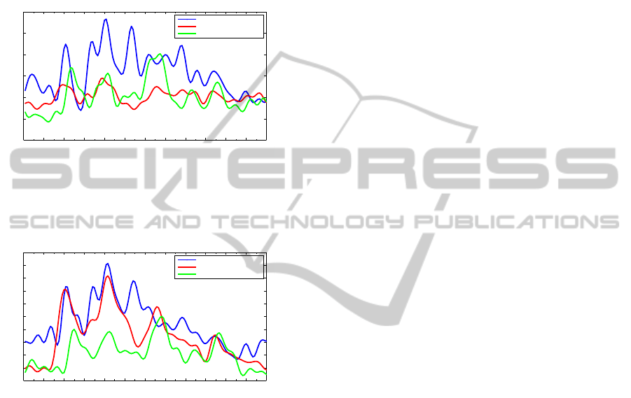
According to (Chrousos, 1998) the frequency of
the ultradian oscillations is rather insensitive to stress
whereas the amplitude increases. Examples of data
for normal and depressed subjects (diagnosed by psy-
chiatrists) showing circadian and ultradian oscilla-
tions are illustrated in figure 1 and figure 2.
0 120 240 360 480 600 720 840 960 1080 1200 1320 1440
0
10
20
30
40
50
60
Time [min]
ACTH concentration[pg/ml]
Hypercortisol depressive
Normal
Lowcortisol depressive
Figure 1: Example of filtered ACTH data of three individ-
uals from the hypercortisol depressed group, the low corti-
sol depressed group and a normal person. Time t=0 corre-
sponds to midnight. Data was sampled every tenth minutes
through 24 hours.
0 120 240 360 480 600 720 840 960 1080 1200 1320 1440
0
2
4
6
8
10
12
14
16
18
20
Time [min]
Cortisol concentration[µg/dl]
Hypercortisol depressive
Normal
Lowcortisol depressive
Figure 2: Example of filtered cortisol data corresponding
to the individuals represented in figure 1. Time t=0 corre-
sponds to midnight. Data was sampled every tenth minutes
through 24 hours.
Understanding the interplay between the various
elements of the HPA axis is interesting and important.
Since several feedback mechanisms are working si-
multaneously in the HPA axis cause and effect may be
hard to distinguish. A mathematical model may help
understand this and can be an important tool for point-
ing out different ways in which malfunctioning may
occur. More specifically, if we are able to estimate
parameters based on a correct model of the HPA axis
and individual data, i.e. concentrations of the hor-
mones ACTH and cortisol in blood plasma samples,
and some of these parameters varies significantly be-
tween groups of depressed subjects and normal sub-
jects, then these parameters characterise the state of
the disease and at the same time pinpoint the mecha-
nisms which are malfunctioning.
2 MODELS OF THE HPA AXIS
It is commonly known that cortisol inhibits the secre-
tion of CRH through glucocorticoid receptors (GR)
situated in the hypothalamus (Wilson and Foster,
1992). In addition cortisol also performs a negative
feedback on the secretion of ACTH through GR situ-
ated in pituitary (Tortora and Derrickson, 2006). This
description is called ’the minimal model of the HPA-
axis’ and has been thoroughly investigated in (Vinther
et al., 2011). In (Vinther et al., 2011) as well as
in (Kyrylov et al., 2004; Kyrylov et al., 2005; Jelic
et al., 2005; Savic and Jelic, 2005; Savic and Jelic,
2006; Liu et al., 1999; Bingzhenga et al., 1990) the
splitting of the circadian and ultradian rhythm is as-
sumed. This is in such a way that the ultradian rhythm
is considered an inherent behaviour of the HPA axis
whereas the circadian rhythm is thought of as an ex-
ternal input to the axis. The models presented in
(Vinther et al., 2011; Kyrylov et al., 2004; Kyrylov
et al., 2005; Jelic et al., 2005; Savic and Jelic, 2005;
Savic and Jelic, 2006; Liu et al., 1999; Bingzhenga
et al., 1990) all consist of a system coupled non-linear
ordinary differential equations. Despite different ap-
proaches the common aim of these publications is
to have unstable and oscillating solution curves. In
(Vinther et al., 2011; Savic and Jelic, 2005; Savic
and Jelic, 2006) this was done by looking for a Hopf-
bifurcation of a stable fixed point, thus guaranteeing
oscillating solutions. However previous results docu-
mented in (Vinther et al., 2011) was that this ’minimal
model of the HPA axis’ was not capable of reproduc-
ing the characteristics seen in data using reasonable
parameter values. This suggests that the ultradian os-
cillations arise from other mechanisms like bursting
which has been investigated successfully by (Veld-
huis et al., 1989; Keenan et al., 2001; Keenan and
Veldhuis, 2003). It has also been suggested that the
ultradian oscillations may arise from the introduction
of a time delay (Vinther et al., 2011; Bairagi et al.,
2008). However, investigations show that rather large
time-delays (i.e. at least 18 minutes) in the feedback
mechanisms are needed (Vinther et al., 2011). Fur-
thermore, one might suggest that the ultradian oscil-
lations are not an inherent behaviour of the HPA-axis
but imposed from outside. A last possibility is that
something is missing in the minimal description of
the HPA-axis. In the latter case, we have suggested
the inclusion of mechanisms from hippocampus, see
(Andersen et al., 2010; Andersen et al., 2013).
2.1 Inclusion of Hippocampal Dynamics
It has been suggested that hippocampus is also play-
PatientSpecificModellinginDiagnosingDepression-CombiningMixtureandNon-linearMixedEffectModelling
659

ing a role for the dynamics of the HPA axis in such
a way that hippocampus stimulates hypothalamus to
produce CRH (Jelic et al., 2005; de Kloet et al., 1998;
Jacobson and Sapolsky, 1991; Oitzl et al., 1995). Fur-
thermore cortisol should be able to exert a feedback
on mineralcorticoid receptors (MR) and GR situated
in hippocampus. More specific cortisol should exert a
positive feedback through GR in hippocampus and a
negative feedback through MR in hippocampus (Jelic
et al., 2005; Oitzl et al., 1995).
To our knowledge there is no known hormone se-
creted from hippocampus to stimulate secretion of
CRH from hypothalamus neither does data for con-
centration of CRH exist for humans. Therefore one
is faced with the challenge of how to model the hip-
pocampal dynamics. The amount of cortisol binding
to MR compared to the amount binding to GR deter-
mines whether the inclusion of hippocampal mecha-
nisms corresponds to a positive or negative feedback.
However this may depend on the concentration of cor-
tisol thus given a positive feedback for some concen-
trations and a negative for others.
The inclusion of a competing positive and neg-
ative feedback mechanism widens the possible be-
haviour of the model compared to a purely negative
feedback model. The idea is that the inclusion of hip-
pocampal mechanisms would give an unstable fixed
point that could explain the ultradian oscillations seen
in data.
The known features the model reflects are feed-
back from cortisol on the secretion of CRH and
ACTH and the combined feedback effect from hip-
pocampus. Since no known hormone is secreted from
hippocampus the known features from hippocampus
is directly included in the differential equation gov-
erning CRH. This approach leads to the model given
in equations (1) - (3) and is denoted the general
model,
dx
1
dt
= f
1
(x
3
) − w
1
x
1
, (1)
dx
2
dt
= f
2
(x
3
)x
1
− w
2
x
2
, (2)
dx
3
dt
= k
2
x
2
− w
3
x
3
. (3)
The overall feedback from cortisol (x
3
) in hippocam-
pus and on CRH (x
1
) is modelled through the func-
tion f
1
(x
3
). The negative feedback from corti-
sol on ACTH (x
2
) is modelled through the func-
tion f
2
(x
3
). w
1
, w
2
, w
3
are elimination constants and
w
1
, w
2
, w
3
> 0, f
1
, f
2
: R
+
∪{0} 7→ R
+
∪{0}, f
1
, f
2
∈
C
1
, sup( f
1
) = M
1
∈ R
+
, sup( f
2
) = M
2
∈ R
+
,f
1
(0) >
0 and f
2
(0) > 0. This means f
1
and f
2
are bounded
functions mapping non negative real numbers into
non negative real numbers. f
1
and f
2
have non neg-
ative domains since the cortisol concentration is non
negative. The ranges of f
1
and f
2
are non negative
since the positive stimulation of the hormones must
not turn negative. The criteria that f
1
and f
2
are
bounded reflects the saturation of receptors through
which the feedbacks are realized. When no cortisol is
present the feedbacks must not completely shut down
the stimulation of hormone production. This justifies
f
1
(0) > 0 and f
2
(0) > 0. It is further assumed that the
feedback on ACTH is negative meaning f
′
2
(x
3
) < 0,
∀x
3
∈ R
+
∪{0}. An approach similar to this has been
investigated by (Conrad et al., 2009). However, in
(Conrad et al., 2009) the ACTH and CRH compart-
ment are pooled together.
The major conclusions (see (Vinther et al., 2011;
Andersen et al., 2010; Andersen et al., 2013)) con-
cerns the possibility of oscillating solutions:
• For the general model there exist a trapping re-
gion. This means that all solutions are guaranteed
not to become negative or tend to infinity.
• The characteristic ultradian oscillations seen in
data has been suggested to be an inherent be-
haviour of the HPA-axis. However the general
model is not capable of giving oscillating solu-
tions within physiologically reasonable parameter
values. This suggests that origin of the ultradian
rhythm should be found in different mechanisms
than the ones included in the general model.
• Using the default parameters the system is glob-
ally stable. This means that the solution curves
will converge to a unique fixed point for all ini-
tial conditions. This can be interpreted as healthy
people returns to normal cortisol levels after peri-
ods of stress.
• A perturbation of the parameters may lead to bi-
furcations where the system undergo a transition
from having a unique stable fixed point to hav-
ing three fixed points where one is unstable and
the two others are stable. All solution curves con-
verge to one of the two stable fixed points depend-
ing on the initial conditions. This is accordance
with the fact that depressed individuals is either
hypercortisolemic depressive or hypocortisolemic
depressive.
In the following we will pose a novel model ex-
tending the general model capable of showing both
circadian as well as ultradian oscillations.
2.2 A Novel Model of the HPA Axis
The fundamental extension from earlier, e.g. equa-
tions (1) - (3), is that we allow a positive (super-short)
feedback in hypothalamus, i.e. from CRH on its own
SIMULTECH2013-3rdInternationalConferenceonSimulationandModelingMethodologies,Technologiesand
Applications
660

production. However, this is not based on pure specu-
lation but on experimental evidence, see (Motta et al.,
1970; Louis et al., 1987; Zanisi et al., 1987). In com-
parison with most specific models in the literature an-
other novelty is the inclusion of non-linear terms in
the feedbacks and the feedforwards (i.e. the terms x
2
3
and x
2
2
) thus large concentration of ACTH and cortisol
affects the production of cortisol and CRH, respec-
tively, more pronounced than linear terms.
Hence we propose the improved novel model,
dx
1
dt
= C(t)
a
1
+ a
2
x
1
1+ a
3
x
3
+ a
4
x
2
3
− w
1
x
1
, (4)
dx
2
dt
=
a
5
x
1
1+ a
6
x
3
− w
2
x
2
, (5)
dx
3
dt
= a
7
x
2
+ a
8
x
2
2
− w
3
x
3
. (6)
Here the circadian rhythm is generated by the endoge-
nous input
C(t) = t
3
m
exp(−
t
m
120
), (7)
where t
m
denotes time t modulo 24 hours (the time
units used is minutes).
3 METHODS
Models should be developed so they incorporate the
responsible mechanisms for the modelled phenom-
ena, i.e. they should be mechanisms-based and they
should be based on first principles (conservationlaws,
etc.) whenever possible. Thus mechanisms-based
models may be rather detailed models. Somehow in
oppose to this demand but in order to identify and es-
timate patient-specific parameters in an effective and
reliable way, the number of parameters has to be kept
as low as possible, which means that any unimpor-
tant factors and elements should be excluded. Hence
a compromise between these conflicting demands of-
ten result in models based on elements resembling the
underlying mechanisms as well as lumped elements.
In any case, all parameters should have physiological
interpretations. Following the principle of parsimony
a model should be as simple as possible fulfilling the
purpose of the modelling task without contradicting
existing knowledge. This has been the guidance in
deriving the novel model presented in section 2.2.
Patient-specific models are (preferable
mechanisms-based) models with physiologically
interpretable parameters related to different patholo-
gies and healthy states in which the values of the
parameters can be individually estimated. Thus,
patient-specific models are models that can be
adjusted to specific individuals. Hence, in patient-
specific models, pathologies are clarified by the
values of certain parameters. The parameters are
estimated from measurements in combination with
the model, thus giving rise to more precise clinical
diagnoses and more reliable suggestions for treat-
ments than are known based on today’s practices. In
addition, existing classes of diagnosed cases may be
refined into subclasses of pathologies corresponding
to the actual defect of the physiological system
by use of such patient-specific models. Moreover,
knowing the actual defect(s) makes the develop-
ment of target-specific drugs and other treatments
possible. Development of this kind can guide the
pharmaceutical industry in its search for new and
improved drugs. In addition, a huge reduction in the
cost of developing new drugs may be expected not
only due to a more beneficial process when searching
for drug candidates but also because models may be
used to substitute some costly animal and human
experiments in future pre-clinical and clinical trials,
respectively.
The parameters have to be estimated by statisti-
cally founded algorithms (for example, the extended
Kalman filter, the Nelder-Mead algorithm combined
with simplex methods, multidirectional search, par-
ticle filter/sequential Monte Carlo methods, genetic
algorithms, Bayesian methods etc.) or by functional
analysis, i.e. optimal control, functional differential
analysis, collocation methods, etc. Not all the pa-
rameters will necessarily be identifiable due to lim-
itations concerning available data and/or an over-
parameterization of the model. Thus, the estimation
process has to be an iterative procedure coupled with
sensitivity analyses or generalized sensitivity analy-
ses combined with subset selection strategies, for in-
stance.
Presently we are examine how well the shuffled
complex evolution (SCE) algorithm do in estimat-
ing parameters and are about to do the same using
the Metropolis-Hastings Algorithm of the Bayesian
Markov Chain Monte Carlo (MCMC) method and the
iteratively refined pricipal differentialanalysis (iPDA)
also denoted approximated maximum likelihood esti-
mate (AMLE).
When well-validated models with patient-specific
estimated parameters exist, the identification of po-
tential biomarkers becomes achievable. Potentially
parameter estimation by patient-specific models may
identify windows for parameter values defining dif-
ferent states for patients, e.g diseased or healthy. This
would be a big step forward for healthcare compared
with empirical developed biomarkers, since the for-
mer also pinpoint the pathological part of the system
PatientSpecificModellinginDiagnosingDepression-CombiningMixtureandNon-linearMixedEffectModelling
661
0 200 400 600 800 1000 1200 1400
0
2
4
6
8
10
12
14
16
18
20
Time t [min]
CRH [pg/ml]
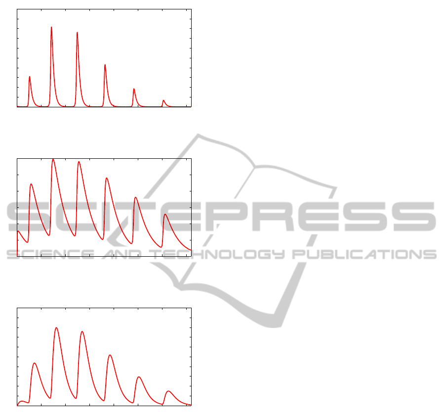
Figure 3: Example of simulated CRH concentration for an
individual.
0 200 400 600 800 1000 1200 1400
0
10
20
30
40
50
60
Time t [min]
ACTH [pg/ml]
Figure 4: Example of simulated ACTH concentration for an
individual.
0 200 400 600 800 1000 1200 1400
0
2
4
6
8
10
12
14
16
18
20
Time t [min]
Cortisol [pg/ml]
Figure 5: Example of simulated cortisol concentration for
an individual.
for diseased patients. When such potential biomark-
ers are identified, different groups of patients, i.e.
pathological subjects versus non-pathological sub-
jects, can be examined. Notice that, some of the pa-
rameters between two different groups have to vary.
To determine whether there is a real difference be-
tween the values of the parameters (i.e. the biomark-
ers) within two groups or whether suggested biomark-
ers can identify variant causes (i.e. pathologies) of the
illness (diagnosed by symptoms), statistical tests have
to be performed. The biomarkers will definitely give
rise to a classification of variants of the illness be-
cause they have inherent features that are naturally in
accordance with data from clinical diagnoses.
4 RESULTS
The values of the 11 parameters of the model pre-
sented in section 2.2 are initially guessed to be a
1
=
4.6, a
2
= 7.6, a
3
= 2.0, a
4
= 0.5, w
1
= 0.34, a
5
=
0.126, a
6
= 3.0, w
2
= 0.011, a
7
= 0.064, a
8
= 0.0165
and w
3
= 0.057. In the near future the parameters will
be estimated by a Bayesian MCMCM method as de-
scribed in section 3 using these parameter values as
initial guesses. The outcome is shown on figures 3, 4
and 5
5 CONCLUSIONS
Depression is a very common disease. Approximately
10% of people in the Western world experience se-
vere depression during their lifetime and many more
experience a mild form of depression. Endocrine
pathologies are believed to be responsible for depres-
sion as well as for stress. Patient-specific modelling
has shown its ability to make diagnoses more precise
and to offer individual treatment plans and drug de-
sign. Efficient and reliable methods for parameter es-
timation are crucial. We have proposed a novel model
capable of showing both circardian as well as ultra-
dian oscillations. These patterns imitate those ob-
served in the correspondingdata. Presently we are ex-
amine how well the shuffled complex evolution (SCE)
algorithm do in estimating parameters. The SCE al-
gorithm is a stepwise global method where a num-
ber of complexes in each step make use of the sim-
plex algorithm and transition between steps evolve
according to a random procedure. The next step is
to investigate which parameters there are responsi-
ble for which pathologies by non-linear mixed effect
(NLME) modelling and statistical hypothesis testing
(ANOVA). Preliminary results are promising. Fi-
nally, we plan to investigate how well the Metropolis-
Hastings Algorithm of the Bayesian Markov Chain
Monte Carlo (MCMC) method for estimating the pa-
rameters is working and we are about to do the same
using iteratively refined principal differential analysis
(iPDA) or the approximated maximum likelihood es-
timate (AMLE).
REFERENCES
Andersen, M., Vinther, F., and Ottensen, J. (2013). Math-
ematical modelling of the hypothalamic-pituritary-
adrenal gland (hpa) axis: Including hippocampal
mechanisms. Mathematical Biosciences.
SIMULTECH2013-3rdInternationalConferenceonSimulationandModelingMethodologies,Technologiesand
Applications
662

Andersen, M., Vinther, F., and Ottesen, J. T. (2010). Global
stability in a dynamical system with multiple feedback
mechanisms. Submitted.
Bairagi, N., Chatterjee, S., and Chattopadhyay, J. (2008).
Variability in the secretion of corticotropin-releasing
hormone adrenocortcotropic hormone and cortisol
and understanding of the hypothalamic-pituitary-
adrenal axis - a mathematical study based on clini-
cal evidence. Mathematical Medicine and Biology,
25:37–63.
Bingzhenga, L., Zhenye, Z., and Liansong, C. (1990). A
mathematical model of the regulation system of the
secretion of glucocorticoids. Journal of Biological
Physics, 17(4):221–233.
Carroll, B. J., Cassidy, F., Naftolowitz, D., Tatham, N. E.,
Wilson, W. H., Iranmanesh, A., Liu, P. Y., and Veld-
huis, J. D. (2007). Pathophysiology of hypercorti-
solism in depression. Acta Psychiatrica Scandinavia,
115.
Chrousos, G. (1998). Editorial: Ultradian, circadian,
and stress-related hypothalamic-pituitary-adrenal axis
activity- a dynamic Digital-to-Analog modulation.
Endocrinology, 139.
Conrad, M., Hubold, C., Fischer, B., and Peters, A. (2009).
Modeling the hypothalamus-pituitary-adrenal system:
homeostasis by interacting positive and negative feed-
back. J Biol Phys, 35.
de Kloet, E. R., Vreugdenhil, E., Oitzl, M. S., and Joels,
M. (1998). Brain Corticosteroid Receptor Balance in
Health and Disease. Endocr Rev, 19(3):269–301.
Griffin, J. E. and Ojeda, S. R. (2004). Textbook of Endocrine
Physiology, Fifth Edition. Oxford University Press,
Inc.
Jacobson, L. and Sapolsky, R. (1991). The role of the hip-
pocampus in feedback regulation of the hypothalamic-
pituitary-adrenocortical axis. Endocr Rev, 12(2):118–
134.
Jelic, S., Cupic, Z., and Kolar-Anic, L. (2005). Mathemat-
ical modeling of the hypothalamic-pituitary-adrenal
system activity. Mathematical Biosciences, 197.
Keenan, D. M., Licinio, J., and Veldhuis, J. D. (2001).
A feedback-controlled ensemble model of the stress-
responsive hypothalamo-pituitaryadrenal axis. Proc.
Natl. Acad. Sci. USA, 98(7):4028–4033.
Keenan, D. M. and Veldhuis, J. D. (2003). Cortisol feed-
back state governs adrenocorticotropin secretory-burst
shape, frequency, and mass in a dual-waveform con-
struct: time of day-dependent regulation. Am J Phys-
iol Regul Integr Comp Physiol, 285:950–961.
Kyrylov, V., Severyanova, L. A., and Vieira, A.
(2005). Modeling robust oscillatory behaviour of the
hypothalamic-pituitary-adrenal axis. IEEE Transac-
tions on Biomedical Engineering, 52.
Kyrylov, V., Severyanova, L. A., and Zhiliba, A. (2004).
The ultradian pulsatility and nonlinear effects in the
hypothalamic-pituitary-adrenal axis. The 2004 Inter-
national Conference on Health Sciences Simulation
(HSS 2004), San Diego, California.
Liu, Y.-W., Hu, Z.-H., Peng, J.-H., and Liu, B.-Z. (1999).
A dynamical model for the pulsatile secretion of the
hypothalamo-pituary-adrenal axis. Mathematical and
Computer Modelling, 29(4):103–110.
Louis, V., King, R., and AJ., C. (1987). In vivo and in
vitro examination of an autoregulatory mechanism for
luteinizing hormone-releasing hormone. Endocrinol-
ogy, 120:272–279.
Motta, M., Piva, F., and Martini., L. (1970). In Martini,
L. e. a., editor, In The Hypothalamus, page 463, New
York. Academic Press.
Oitzl, M. S., van Haarst, A. D., Sutanto, W., and de Kloet,
E. R. (1995). Corticosterone, brain mineralocorticoid
receptors (mrs) and the activity of the hypothalamic-
pituitary-adrenal (hpa) axis: The lewis rat as an exam-
ple of increased central mr capacity and a hyporespon-
sive hpa axis. Psychoneuroendocrinology, 20(6):655
– 675.
Savic, D. and Jelic, S. (2005). A mathematical model of
the hypothalamo-pituitary-adrenocortical system and
its stability analysis. Chaos, Solitons & Fractals, 26.
Savic, D. and Jelic, S. (2006). Stability of a general de-
lay differential model of the hypothalamo-pituitary-
adrenocortical system. International Journal of Bi-
furcation and Chaos, 16.
Tortora, G. J. and Derrickson, B. (2006). Principles of
Anatomy and Physiology, 11th edition. John Wiley
& Sons, Inc.
Veldhuis, J. D., Iranmanesh, A., Lizarralde, G., and John-
son, M. L. (1989). Amplitude modulation of a burst-
like mode of cortisol secretion subserves the circa-
dian glucocorticoid rhythm. Am J Physiol Endocrinol
Metab, 257:6–14.
Vinther, F., Andersen, M., and Ottesen, J. T. (2011). The
minimal model of the hypothalamic-pituitary-adrenal
axis. Journal of Mathematical Biology, 63(4):663–
690. (Epub Nov 24, 2010). Resubmitted.
Wilson, J. D. and Foster, D. W. (1992). Williams Textbook of
Endocrinology, Eighth Edition. W. B. Saunders Com-
pany.
Zanisi, M., Messi, E., Motta, M., and Martini., L. (1987).
Ultrashort feedback control of luteinizing hormone-
releasing hormone secretion in vitro. Endocrinology,
121:21992204.
PatientSpecificModellinginDiagnosingDepression-CombiningMixtureandNon-linearMixedEffectModelling
663
