
A Spiking Neuron Model based on the Lambert W Function
Yevgeniy Bodyanskiy and Artem Dolotov
Control Systems Research Laboratory, Kharkiv National University of Radio Electronics, 14 Lenin Ave., Kharkiv, Ukraine
Keywords: Self-learning Spiking Neural Network, Spiking Neuron, Lambert W Function, Postsynaptic Potential,
Membrane Potential.
Abstract: A model of spiking neuron based on the Lambert W function has been proposed. It is shown analytical
dependence of spiking neuron firing time on input spikes can be obtained. Though such dependence is
rather complex, it still allows of simplifying software implementation of spiking neural networks. It is
demonstrated the proposed model software implementation operates faster than one of straightforward
propagation of a spike through multiple synapse and soma of spiking neuron.
1 INTRODUCTION
From the software implementation standpoint, of
greater importance is analytical representation of
spiking neuron firing time dependence on input
spikes inasmuch as firing time holds a central
position both in conventional self-learning spiking
neural networks (as a parameter to determine cluster
that the input pattern belongs to (Natschlaeger and
Ruf, 1998)) and in hybrid systems based on them (as
a distance between input pattern and clusters, that is
utilized for fuzzy partitioning (Bodyanskiy and
Dolotov, 2009)). Such dependence has not been
obtained till now so, when implementing a software
model of spiking neural network, a researcher has to
emulate dynamics of spiking neuron soma
membrane potential in order to determine
empirically the moment when it crosses firing
threshold, which differs radically from conventional
artificial neural networks where a neuron output is
readily expressed on its inputs. Considering
population coding is usually used in self-learning
spiking neural networks (Bohte et al., 2002), and
their synapses are compound structures (Gerstner
and Kistler, 2002) – so even one input gives rise to a
set of spikes that come to soma via different paths,
software applications based on spiking neural
networks may operate significantly slowly because
of necessity to emulate spiking neuron membrane
potential dynamics.
In the next sections, it is shown that output spike
firing time dependence on incoming spikes may be
expressed analytically based on the Lambert W
function and thus the mentioned difficulty in spiking
neural networks implementation may be overcome.
Performance of the proposed model of spiking
neuron is compared with one of a straightforward
model of spiking neuron.
2 ANALYTICAL DEPENDENCE
OF SPIKING NEURON FIRING
TIME ON INPUT SPIKES
In order to obtain an analytical dependence of
spiking neuron firing time on input spikes, let us
solve the simpler task first: obtaining firing time of a
spiking neuron when it receives one incoming spike
(we will use ‘conventional’ architecture of self-
learning spiking neural network introduced in
(Bohte et al., 2002)).
Spiking neuron receives input signal in a pulse-
position form (incoming spikes), transforms it into
continuous-time form (membrane potential), and
transforms it back to pulse-position form on its
output (outgoing spike). Let us examine such
transformation using spiking neuron j with a simple
(not multiple) synapse without time delay that
connects the i-the neuron of the previous layer (it
may be either a receptive neuron or a spiking
neuron) with the neuron. Its membrane potential is
ijij
ttwtu
)( ,
(1)
i
ii
i
ttH
tttt
tt
1exp
(2)
542
Bodyanskiy Y. and Dolotov A..
A Spiking Neuron Model based on the Lambert W Function.
DOI: 10.5220/0004631605420546
In Proceedings of the 5th International Joint Conference on Computational Intelligence (NCTA-2013), pages 542-546
ISBN: 978-989-8565-77-8
Copyright
c
2013 SCITEPRESS (Science and Technology Publications, Lda.)

where
i
t is a spike produced by the i-th neuron,
ji
w
is a synaptic weight between the i-th and the j-th
neurons,
ε is a spike-response function,
is the
membrane potential decay time constant,
H is
the Heaviside step function. At the moment when
)(tu
j
reaches firing threshold
s.n.
, the spiking
neuron generates outgoing spike
j
t on its output.
The task is to find dependence
)(
ij
tt .
In order to solve the problem, we have to utilize
the function that is inverse to function
z
zezf )(
(3)
where z is a complex variable. Plot of function
)(zf
is depicted on Figure 1.
-8 -7 -6 -5 -4 -3 -2 -1 0
-0.4
-0.3
-0.2
-0.1
0
0.1
0.2
0.3
0
.
4
Figure 1: Function
z
zezf )(
.
The inversion function of )(zf is the Lambert W
function, also called the omega function,
)(z
(Corless, Gonnet, Hare, et al., 1996). It cannot be
expressed in terms of elementary functions. It has
two main branches on interval
0,
1
e
(Figure 2):
)(
1
x
when 1)(
x (dashed line) and
)(
0
x when 1)( x (solid line).
Let us solve now the equation
s.n.
)(
tu
j
(4)
for t (t is apparently less than simulation interval
time
sim
t ). Using (1), (2), and the Heaviside step
function definition, we can express membrane
potential of the j-th neuron as follows:
.,0
;,
1
i
i
tt
i
ji
j
tt
tte
tt
w
tu
i
(5)
Case
i
tt doesn’t make sense as a spiking neuron
can’t fire until the only incoming spike
i
t reaches it
so the equation (4) takes from
s.n.
1
i
tt
i
ji
e
tt
w .
(6)
-0.4 -0.3 -0.2 -0.1 0 0.1 0.2 0.3 0.4
-8
-7
-6
-5
-4
-3
-2
-1
0
Figure 2: Function )(x .
It should be noted that, from practical
considerations, parameters of equation (6) may be
bounded as follows:
0
ji
w ,
(7)
0
,
(8)
0
s.n.
.
(9)
Now, applying definition of
)(
0
x (as we aim to
get time when membrane potential crosses firing
threshold from below), we obtain
ji
i
ew
tt
s.n.
0
(10)
or
ji
ij
ew
ttt
s.n.
0
.
(11)
Let us consider now more complex case when two
spikes
1
t and
2
t generated by neurons of the
previous layer reach the
j-th spiking neuron, and the
first neuron in the previous layer has fired earlier
than the second one, i.e.
21
tt
. (12)
Equation (4) will take the following form in such
case:
s.n.2
1
2
2
1
1
1
1
2
1
ttHe
tt
w
ttHe
tt
w
tt
j
tt
j
(13)
ASpikingNeuronModelbasedontheLambertWFunction
543

or in an expanded form:
.,,
,
;,
,
;,
,
;,
,0
sim21
s.n.
1
2
2
1
1
1
21
s.n.
1
1
1
21
s.n.
1
2
2
21
s.n.
21
1
2
tttttt
e
tt
we
tt
w
tttt
e
tt
w
tttt
e
tt
w
tttt
tt
j
tt
j
tt
j
tt
j
(14)
Taking into account (9) and (12), the first and the
second systems of equations from (14) do not make
sense. Solution of the third system of equations is
similar to (11), namely
1
s.n.
01
j
j
ew
ttt
.
(15)
By solving the fourth system of equations from (14),
we obtain the following dependence
.
21
2
2
1
1
2
22
1
11
21
21
21
s.n.
0
21
2211
t
j
t
j
ewew
etwetw
t
j
t
j
t
j
t
j
ewew
e
e
ewew
etwetw
t
t
j
t
j
t
j
t
j
(16)
It is notable that equation (16) is substantially
generalization of equation (15): it defines a wave
whose inverse form is identical to a separate
postsynaptic potential and that considers effect of
the preceding spike on the neuron’s membrane
potential.
3 A SPIKING NEURON MODEL
Let us generalize equation (16) now for case of
arbitrary number of incoming spikes.
It is worthy of note that solution (15), (16) of
equation (13) defines two time intervals –
21
,tt
and
sim2
,tt where on each interval, membrane
potential of spiking neuron’s soma takes wave-like
form that is caused by two incoming spikes.
Utilizing
)(
0
x
in (15), (16), we consider on the
mentioned interval only those lapses where
membrane potential monotonically increases since
we need to obtain moment when membrane potential
reaches firing threshold from below. Solution (15),
(16) gives firing time of neuron when its membrane
potential reaches firing threshold either on the
interval when its value monotonically increases for
the first time (soma receives incoming spike
1
t
) or
on the interval when it increases for the second time
(soma receives incoming spike
2
t ). If solution (15)
does not produce a real value, it means the
membrane potential has not reached firing threshold
still so the second interval should be analyzed. If
solution (16) has not produces a real value either, it
means two incoming spikes are not sufficient to fire
the neuron.
Evidently the reasoning above may be applied to
arbitrary number of incoming spikes so in order to
obtain a generalized solution, we have to analyze
each interval one by one where membrane potential
increases to find the first moment when it reaches
firing threshold. Such exhaustive search apparently
requires much less number of comparisons as
opposed to continual comparing on each time step in
straightforward modelling of spiking neurons. To
perform the comparison, all spikes incoming to the
j-
th neuron should be arranged in order of firing time
magnitude (so the set of incoming spikes
niitttT
jiji
,1,0|
max
where
max
t is the latest
possible firing time of neuron of the previous layer,
n is the number of neurons in the previous layer,
should be transformed to linearly ordered set
niiTtttt
ijijijij
,1
ˆ
,
ˆ
,|
ˆˆ
1
ˆ
,
ˆ
). Then the
simulation interval should be broken down with
respect to the ordered set of incoming spikes
(intervals
sim
ˆ
1
ˆ
,
3,2,2,1,
,...,,...,,,, tttttttt
jn
ijij
jjjj
).
Finally, each interval should be analyzed
sequentially whether membrane potential reached
firing threshold – once the first real value is
obtained, the search should be stopped.
By increasing number of addends to current
number of intervals that have been analyzed, we can
generalize equations (15), (16) as follows:
B
e
eB
A
tt
B
A
j
s.n.
0
,
(17)
kj
t
kj
i
k
kj
ewtA
ˆ
ˆ
ˆ
1
ˆ
ˆ
,
(18)
IJCCI2013-InternationalJointConferenceonComputationalIntelligence
544

i
k
t
kj
kj
ewB
ˆ
1
ˆ
ˆ
ˆ
.
(19)
where
i
ˆ
is the number of interval currently being
analyzed;
kj
t
ˆ
is an enumerated spike,
kj
w
ˆ
is a
weight of synapse that spikes comes to soma
through. Now if one calculates
j
t according to (17)-
(19) on each time interval until a real value is
received, he can obtain spiking neuron firing time
for an arbitrary number of incoming spikes (Figure 3
illustrates case with three incoming spikes).
Thus, having analytical model of spiking neuron,
a researcher can easily implement a software
application of self-learning spiking neural network
(learning procedures of spiking neural networks are
out of scope of this paper). Under easy software
implementation, we understand the fact that a
researcher does not have to program spike
propagation form a receptive neuron or a spiking
neuron through multiple synapse to soma of the
spiking neuron whose firing time is being obtained.
In a sense, the proposed model of spiking neuron is
akin to conventional models of artificial neural
networks of the second generation as they are
constructed in terms of matrix algebra, thus allowing
developers and researcher to avoid biological aspect
of neurons operating.
An additional advantage of the proposed model
is that it can operate in a sequence mode when new
spikes constantly come to spiking neuron inputs.
However, we have to note here that spiking neuron
refractoriness and effect of spike-after potential on
further neuron firing are not considered in this work
as in any case they play no part in the most of
spiking neural networks used in actual practice.
4 SPIKING NEURON SOFTWARE
IMPLEMENTATIONS
PERFORMANCE
Nowadays software applications of the designed
models and systems are in most common use due to
their simplicity and low price as compared to
hardware implementations. This brings up an
important question on performance of different
spiking neuron software implementations.
Surprisingly, ways to improve spiking neural
network models for software implementation are
poorly researched. This section describes results of
performance testing of two spiking neuron software
implementations – straightforward model and the
model introduced in this paper based on the Lambert
W function.
The straightforward model of spiking neuron (an
example of it can be found in (De Berredo, 2005))
emulates spiking neuron membrane potential
dynamics and has to check whether its value crossed
firing threshold on each time step.
Software implementation of the spiking neuron
model introduced on the Lambert W function base
rests on the procedure described in the previous
section: incoming spikes are put in order of their
firing time magnitude and
j
t is calculated with
(17)-(18) on each time interval formed; the first real
value of
j
t indicates firing time of spiking neuron.
As seen from Table 1, the introduced model is
always faster than the straightforward model though
its operating time raises as size of input spikes
vector increases.
Table 1: Results of performance testing of straightforward
model of spiking neuron and the model proposed in this
paper.
Size of input
spikes vector
Firing time calculation speed, s
Straightforward
model
Model based on
the Lambert W
function
10 0.0019 0.0012
50 0.254 0.148
100 0.706 0.308
300 2.129 1.524
500 4.018 1.757
We have to note here that in practice, a range of
various techniques are used to improve performance
of software implementations (e.g., methods of
matrix algebra). We used just ‘pure’ models for the
sake of reference models comparison.
5 CONCLUSIONS
The major conclusion of the research is that
analytical dependence of spiking neuron firing time
on input spikes can be expressed – but in an intricate
way. That fact complicates comprehensive analysis
of spiking neural networks behavior and features.
However, the proposed spiking neuron model allows
of improving spiking neural networks software
implementations performance. It also allows a
researcher to abstract away from biological specific
of spiking neural networks when implementing them
and to use them just as a regular tool for data
processing. Another advantage of the proposed
model is its precision level of the firing time
ASpikingNeuronModelbasedontheLambertWFunction
545
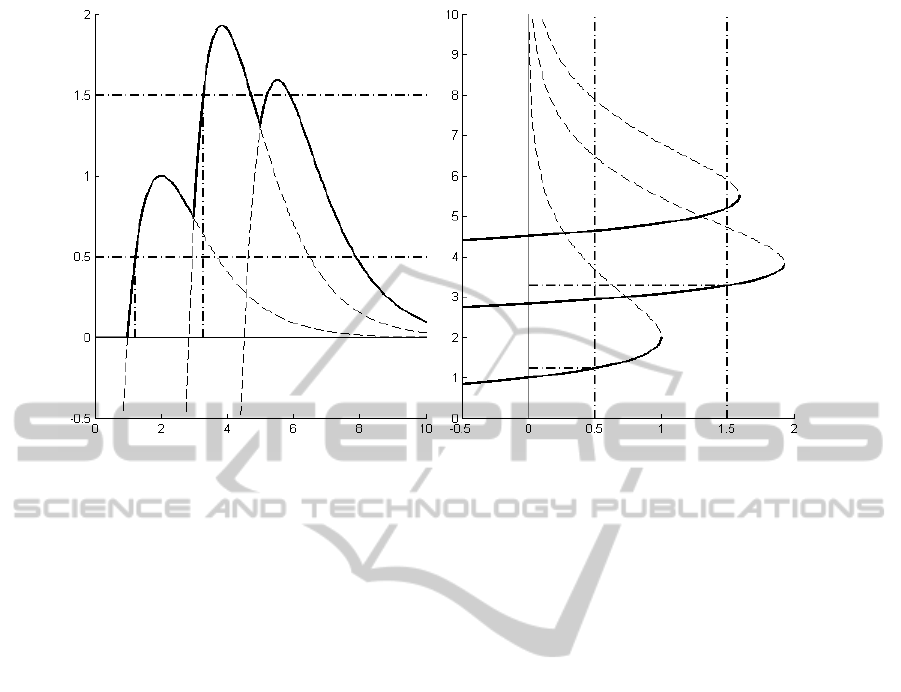
Figure 3: Spiking neuron firing time obtaining in case of three incoming spikes. Left: Spiking neuron soma membrane
potential dynamics caused by incoming spikes (solid line) is presented as a sum of single postsynaptic potentials defined by
spike-response function (2) (dashed line). Two different firing thresholds are marked with horizontal dash-and-dot lines. In
the straightforward model of spiking neuron, neuron firing event occurrence is checked on each sampled time step. Sampled
time when that event occurred defines
j
t (vertical dash-and-dot line). Right: Dependence of
j
t on firing threshold
indicates equation (4) solution based on
)(
0
x
(solid line) and
)(
1
x
(dashed line). Considered firing threshold values
are marked with vertical dash-and-dot lines. In the model based on the Lambert W function, there may be three checks at
most to obtain
j
t . Given firing threshold is 0.5, firing time is obtained on the first step (bottom horizontal dash-and-dot
line), and given firing threshold is 1.5, firing time is obtained on the second step (top horizontal dash-and-dot line).
calculation that is important in fuzzy spiking neural
networks: contrary to the straightforward model
where precision is bounded with the sampled
interval value, precision in the proposed model is
bounded only by precision of the system in the
Lambert W function calculation.
REFERENCES
Bodyanskiy, Ye., Dolotov, A., 2009. Analog-Digital Self-
Learning Fuzzy Spiking Neural Network in Image
Processing Problems. In Image Processing, INTECH.
Vukovar.
Bohte, S. M., Kok, J. S., La Poutre, H., 2002.
Unsupervised clustering with spiking neurons by
sparse temporal coding and multi-layer RBF networks.
In IEEE Transactions on Neural Networks, 13.
Corless, R. M., Gonnet, G. H., Hare, D. E. G., et al., 1996.
On the Lambert W function. In Advances in
Computational Mathematics, 5.
De Berredo, R. C., 2005. A Review of Spiking Neuron
Models and Applications, A dissertation in fulfillment
of the requirements for the degree of Master of
Science. Belo Horizonte.
Gerstner, W., Kistler, W. M., 2002. Spiking Neuron
Models: Single Neurons, Populations, Plasticity,
Cambridge University Press. Cambridge.
Natschlaeger, T., Ruf, B., 1998. Spatial and temporal
pattern analysis via spiking neurons. In Network:
Computations in Neural Systems, 9.
IJCCI2013-InternationalJointConferenceonComputationalIntelligence
546
