
Macroscopic Simulation of Multi-axis Machining Processes
Meysam Minoufekr
1
, Lothar Glasmacher
1
and Oliver Adams
2
1
CAx-Technologies, Fraunhofer-Insitute for Production Technology, Steinbachstr. 17, 52074 Aachen, Germany
2
Chair of Manufacturing Technology, WZL, RWTH Aachen University, Steinbachstr. 19, 52074 Aachen, Germany
Keywords: Geometric Modelling, NC Machining Simulation, Tool/Workpiece Engagement.
Abstract: The machining of safety-critical components, e.g. turbine disks and blades, is expected to meet highest
demands regarding functionality and quality. At the same time, a fast and affordable process design for the
production is a major driver for the economic development of these components. Effective increase in
productivity requires in addition to the development of machining technologies, new approaches in process
design and planning. The integration of simulation into computer aided design of multi-axis processes
provides a great potential for further optimisation of the processes. By using the macro simulation model
introduced in this paper, the computational complexity to gain relevant process information is reduced and
hence made accessible more easily. Through the presented macro simulation, detailed tool-workpiece
engagement is calculated which co-relates to mechanical and thermal stresses on the tool. Based on the
calculations the process can be designed by reducing the tool load in the course of the process. This way, the
tool life of the used milling cutters can be significantly increased resulting in an increase of process
robustness and efficiency, thereby reducing used resources.
1 INTRODUCTION
The process sequence for milling of free-form
surfaces can be divided into roughing, pre-finishing
and finishing. When roughing, the goal is often to
achieve a high performance cutting process (HPC)
by driving the process at maximal feed rates and
depth of cut resulting in a high material removal rate
(MRR). However, in HPC processes high feed rates
lead to increasing cutting forces and tool loads
which have to be controlled in order to avoid a large
tool wear or even tool breakage during the process.
The workpiece resulting from the roughing
operation is usually characterized by a macroscopic
surface roughness on the surface contour, (Arntz,
2013). In pre-finishing, a uniform surface is
achieved by removing the rest material generated in
the rough machining. The goal of pre-finishing is a
constant material distribution on the entire
workpiece, so that in the following finishing
operation, requirements of accuracy and surface
quality can be achieved. As the last process,
finishing is critical since the final surface of the part
is generated. Failures in finish milling lead to
expensive rework or even to scrap generation. Both,
in pre-finishing and in the subsequent finishing
processes, often a high speed cutting (HSC)
approach is applied by using extremely high spindle
speed and feed rates. In the course of HSC
processes, the engagement conditions, e.g. the
contact angle and the resulting chip thickness, have
to be controlled since, in combination with the
cutting speeds, the mechanical and thermal loads on
the tool may result in low surface quality on the final
part. Consequently, in HPC as well as in HSC
processes, methods are needed for a careful process
design to drive the processes to their limits but also
to avoid critical situations along the value chain of
the processes.
Especially in the transition from roughing to pre-
finishing, the analysis and evaluation of the
engagement conditions plays an important role, as
the contact situation between cutter and workpiece
becomes unpredictable. The residual material
geometry on the workpiece, which results from
roughing, usually cannot be determined in advance
for parts with free-form geometry. Contact situations
of the tool and the workpiece leading to unknown
and possibly undesirable engagement conditions
seem to be unavoidable during the process. Due to
the continuously changing machining allowance and
contact situation, it is important for the process
505
Minoufekr M., Glasmacher L. and Adams O..
Macroscopic Simulation of Multi-axis Machining Processes.
DOI: 10.5220/0004631905050516
In Proceedings of the 10th International Conference on Informatics in Control, Automation and Robotics (ICINCO-2013), pages 505-516
ISBN: 978-989-8565-71-6
Copyright
c
2013 SCITEPRESS (Science and Technology Publications, Lda.)
planner to understand the interaction between the
tool and the workpiece and evaluate the same
against significant process parameters. In particular,
the engagement conditions during simultaneous five-
axis milling have to be observed in this context.
The simulation approach introduced in this work
helps to understand the geometrical engagement
situation occurring in the milling process. Thus,
critical regions in the process where engagement
condtions exceed the tolerances can be automatically
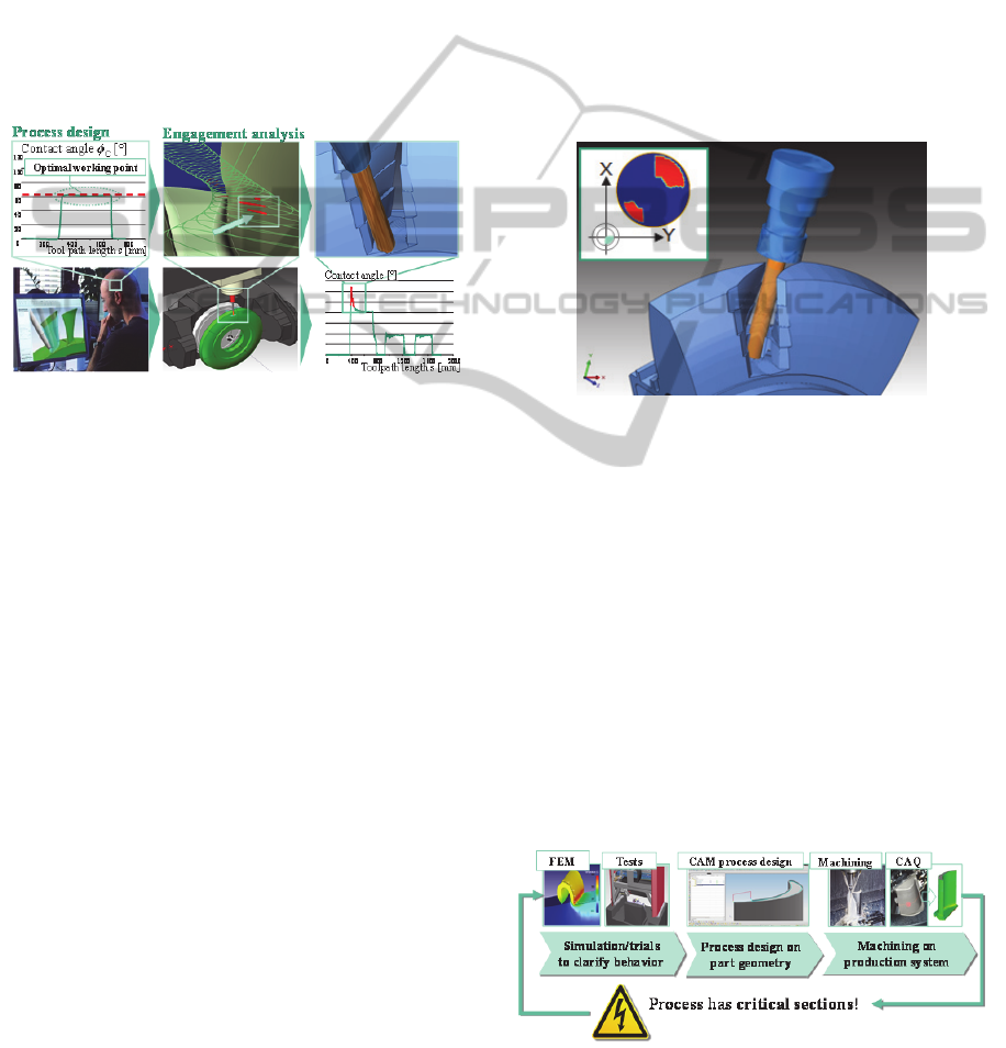
identified, Figure 1. This is the basis for a process
analysis, since process parameters directly related to
the geometrical engagement conditions are evaluated
and optimised in advance.
Figure 1: General idea for simulation of critical sections
on the toolpath.
So, this paper suggests the macro simulation
model for multi-axis machining processes. It is
structured as follows. In section 2, problems in
current multi-axis machining are described.
Furthermore, the engagement and fundamental
parameters defining the cutter-workpiece contact are
analysed. In section 3, the macroscopic simulation
model for machining processes is introduced. Based
on this concept, the calculation models for discrete
engagement conditions are explained in-depth. Then,
in section 4 the macro simulation is discussed by a
roughing example, where engagement conditions are
calculated. The paper is finally concluded in
section 5.
2 BACKGROUND AND
PROBLEM DEFINITION
Almost any complex part can be produced using
simultaneous multi-axis machining. Here, the
simultaneous multi-axis milling is characterized by
suddenly changing the tool orientation and the
transient contact conditions between tool and
workpiece. The manufacturing of the parts is carried
out on NC controlled machine tools. Here, the
process is loaded as a series of NC commands, i.e.
the "NC program", on the machine tool and
executed. Depending on the NC command in the NC
program, up to three translational and two rotational
axes are controlled simultaneously during the
machining. Accurate NC programs are crucial for
manufacturing without interruption and potential
machine breakdowns. Due to the complex
kinematics, milling processes are not verifiable
without supporting process design tools because it is
difficult to visualise the location of the cutting tool
due to the complex axis control. The consequences
are unpredictable and probably critical to cutting
conditions, Figure 2.
Figure 2: Example of a BLISK manufacturing with a
critical engagement due to collision of the workpiece with
the non-cutting part of the cutter.
Nowadays, the development of machining
processes is characterized by a sequential iterative
approach, which has to be followed in a few
optimization loops before reaching stable
production, (Schug, 2012). Therefore, computer
based technologies (CAx technologies) are involved
in planning and verification of the entire milling
process in advance, Figure 3. The parameter
windows and the acquired technology knowledge
gained from machining trials are used to determine
the process-specific, optimal parameter
combinations which are essential in the design and
planning of the manufacturing.
Figure 3: Sequential CAx process chain for machining.
ICINCO2013-10thInternationalConferenceonInformaticsinControl,AutomationandRobotics
506
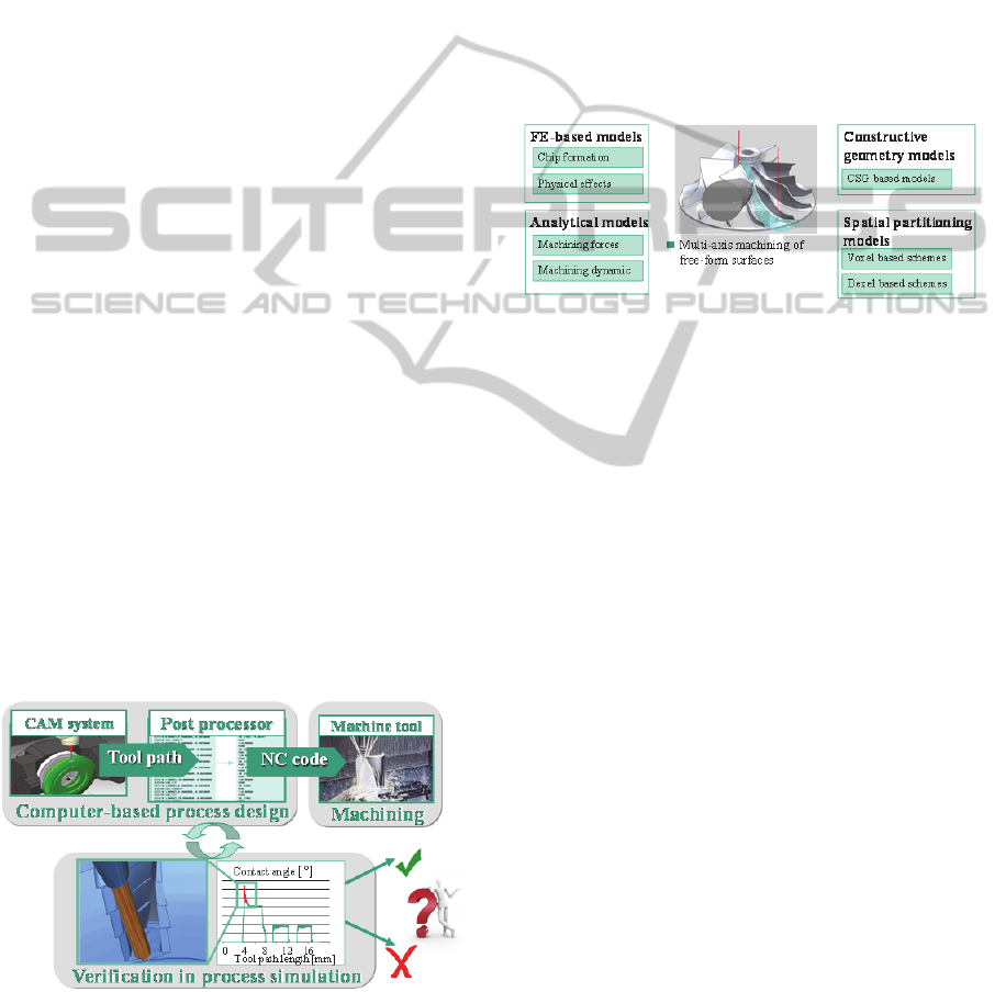
The planning in CAM is dedicated to the design
of the machining operation where the milling
toolpath is parameterized by process variables such
as cutting speed and depth of cut to manufacture the
real part geometry. The designed process is
transferred to the production system by an
appropriate output data format for machining.
Potential errors that are identified at the end of the
process design stage, or during the process carried
out on the machine tool, cause expensive iteration
steps. According to (Zabel, 2010), the costs to
eliminate an error increase with the progress of the
process design stages. Consequently, an
identification of process parameters leading to
undesired cutting conditions is considered necessary
at an early stage in the process planning.
2.1 Simulation-based Design of
Multi-axis Processes
The main application of process simulation is in the
area of computer-based process planning and design,
Figure 4. By using the process simulation, it is
possible to locate errors and fix problems faster, than
it is achievable through trial-and-error methods. The
starting point for using the process simulation
system is between the NC data generation by the
CAx system and the loading of NC data on the
machine tool. Unlike the sequential CAx process
chain, the NC data is not transferred directly to the
machine tool, but passed to the simulation system.
Especially requirements referring to the efficiency of
the used simulation tool process play a role because
the simulation increases the CAx process design
chain length, (Zabel, 2010). In this context, the
simulation model with affordable complexity of
computation time and space is desirable.
Figure 4: Evaluation of the process behaviour by the
presented simulation approach.
2.2 State of the Art in the Simulation of
Machining Processes
Numerous simulation approaches have been
developed in the last decades with the objective of
determining the important parameters of the
machining process which can be classified as FE-
based models, analytical models and geometrical
models, Figure 5. The group of geometrical models
can be further subdivided into approaches using
constructive solid geometries (CSG) and spatial
space partitioning schemes. Zabel gives a detailed
overview of these models and their application in
(Zabel, 2010).
Figure 5: Overview of existing simulation models for
machining processes.
Although many physical effects can be modeled
by using FEM and analytical model equations,
however, the predictive capabilities of available
approaches are still limited and thus cannot be
applied for planning the entire multi-axis operation.
A complete analysis of five-axis milling processes,
i.e. simulation of every instant of the process is
expensive due to limitations on available computing
capacity and hardly practical. On the other hand,
geometric models focus on the determination of
visual properties such as the shape of the workpiece
during the milling operation by efficient real-time
methods for updating the workpiece.
Simulation techniques based on the discretization
of the workpiece vary according to the geometric
design, (Glaeser, 1997), (Jerard, 1989), (Robert,
1987). Milling simulation methods based on the
voxel or dexel model are presented in (Ayasse,
2001) and (Stautner, 2005). The consideration of
physical properties is of minor importance. Systems
like Vericut offer simulation methods for collision
detection in three and five axis milling, (CGTech,
2013). The adjustment of the NC programs is often
based on parameters, wherein the simulated residual
material on the finished part is used to increase the
material removal rate. However, only the feed rates
are adjusted, the geometry of the toolpath remains
unchanged. In these systems, assumptions in the
modeling approaches are highly simplified. Hence,
MacroscopicSimulationofMulti-axisMachiningProcesses
507
results obtained are insufficient for a qualitative
statement about the geometrical engagement
situation in the course of the milling process.
2.3 Macroscopic Engagement
Conditions for Process Evaluation
The mechanical and thermal tool load is primarily
dependent on the combination of three factors: the
chip thickness h
sp
,
the contact angle ϕ
c
and the
contact length l
sp
, Figure 4.
Figure 6: Engagement of cutting tool at instant t.
Optimal cutting conditions can be maintained
easily in straight cuts by constant cutting width a
e
.
However, engagement situations change rapidly in a
multi-axis process. In machining of free-form
surfaces, the contact angle ϕ
c
increases, whenever
the tool enters a turn causing a longer contact length
l
sp
between the cutting edges and the workpiece,
Figure 7. In fact, cutting-edge temperature increases
significantly as the contact length l
sp
increases,
which results in a decrease of tool life. This relation
has been proven by Meinecke in (Meinecke, 2009).
Figure 7: Straight vs. corner cuts result in different
engagement despite equal cutting depth, (Diehl, 2011).
The relevance of the contact angle ϕ
c
can also be
seen in cutting theory, as the chip thickness h
sp
increases with increasing ϕ
c
and thus leads to higher
cutting forces, (Klocke, 2011). According to Ståhl,
(Ståhl, 2012), the approximate chip thickness h
sp
and
the chip width b
sp
are expressed by the contact angle
ϕ
c
and the axial depth of cut a
p
, respectively:
∙
(1)
sin
(2)
where κ is the major cutting edge angle of the
cutting tool, f
z
the feed per tooth and a
p
the cutting
depth. Specifically, the the machining forces in
radial (F
r
), tangential (F
t
) and axial direction (F
a
) are
related to the contact angle ϕ
c
. This can be seen by
substituting h
sp
and b
sp
in the Kienzle equation,
(KLocke, 2011):
F
i
=
a
p
sin
κ
·k
i1.1
·(f
z
·sinϕ
c
)
1-m
i
(3)
where k
i1.1
and m
i
are material specific constants and
i ∈ {a,r,t}. Hence, the contact angle and the contact
length play a major role in the evaluation of
machining processes. For the calculation of the
contact angle ϕ
c
, it is necessary to regard the cutter-
workpiece engagement at each point in time in the
course of the process. However, the contact angle
can be determined by considering the interaction of
the tool bounding geometry with the workpiece,
where the angular contact area on the tool is referred
as ϕ
c
= ϕ
ex
- ϕ
st
, i.e. defined as the difference of the
exiting angle ϕ
ex
and the starting angle ϕ
st
, Figure 8.
In accordance to (Meinecke, 2009), quantities as ϕ
ex
and ϕ
st
are referred to as macro conditions, since
their calculation is abstracted from the exact tool
geometry and the tool cutting edges are not taken
into account.
Figure 8: Macro engagement of cutting tool.
2.4 Influence of the Tool Geometry and
Tool Kinematic
In addition to the suddenly changing contact
situation in the course of the multi-axis milling, two
further aspects complicate the calculation of macro
conditions at each instant of the process; the tool
geometry and tool orientation. During the machining
Engagement on the tool
N
v
f
N
h
sp
b
sp
F
a
F
r
F
t
v
f
y
N
f
z
h
sp
l
sp
=r·ϕ
c
x
ϕ
c
v
f
N
f
z
h
sp
ϕ
c
=60°
a
e
=12%
v
f
N
f
z
ϕ
c
=24°
a
e
=12%
a
p
a
e
v
f
v
c
ϕ
st
·r
ϕ
ex
·r
ϕ
c
·r
l
sp
a
p
ICINCO2013-10thInternationalConferenceonInformaticsinControl,AutomationandRobotics
508
of freeform surfaces many constellations of the
engagement may arise from the material removal
leading to sudden changes of engagement conditions
along the tool.
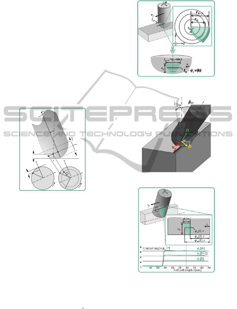
To capture the engagement situation in multi-
axis machining, an extended definition of process
parameters and engagement conditions is needed
considering the tool geometry and the tool
orientation. Hence, the engagement conditions are
parameterized by their axial location k ∈ [0,l] on the
tool axis at an instant in the course of the process.
Thus, the starting and exiting angle are defined as
ϕ
st
(k)
and ϕ
ex
(k), respectively. Also the radial depth
of cut is referred to the current location of the tool
axis and is deifined as a
e
(k). Since the tool radius is
also variable along the tool axis it is also
parameterized as r(k),
Figure
9.
Figure 9: Parameterization of the engagement conditions
in reference to the tool length l.
When machining with ball end mills, for
instance, every cutter point undergoes a different
load during the engagement. The altering contact
along the tool axis has consequences for the
determination of the chip length l
sp
, since it depends
on the contact angle ϕ
c
and tool radius r(k) which is
varying according to the tool shape along the tool
axis,
Figure
10.
The calculation of the engagement condition is
further complicated by the orientation of the tool
relative to the workpiece and the feed direction. In
context of NC machining, the position of the tool is
defined by a local tool coordinate system TCS which
has its origin at the tool center point O
TCS
and is
determined by the current feed direction v
f
, the tool
orientation n and the bi-normal b=n × v
f
,
Figure
11.
The orientation of the tool vector n is determined by
the lead and tilt angle β
fN
and β
N
, respectively.
Figure 10: Influence of the tool geometry on the
calculation of engagement conditions.
Figure 11: Definition of the Tool coordinate system.
Figure 12: Influence of the tool orientation on the
engagement conditions.
During the machining of freeform surfaces, the
tool may be tilted to the surface normal, i.e. β
N
≠0
and β
fN
≠0, respectively. Since the contact situation
depends on the lead angle β
N
and tilt angle β
fN
,
describing the angular situation of the tool normal
vector n to the surface of the workpiece,
v
f
a
e
(k)
ϕ
st
(k)
ϕ
ex
(k)
r(k)
N
NN
a
p
A
A
B
B
B
O
O
O
k
β
fN
MacroscopicSimulationofMulti-axisMachiningProcesses
509
(Arntz, 2013), the starting and exiting angles ϕ
st
(k)
and ϕ
ex
(k) vary along the tool axis resulting from the
kinematic situation of the tool and the workpiece.
Hence, at each individual tool height, there is a
different contact angle ϕ
c
(k), Figure 12. Depending
on the tool orientation to the workpiece, the contact
angle ϕ
c
(k) varies along the tool axis at a discrete
instant t.
2.5 Problem Definition and Research
Question
On one hand, the engagement situation depends on
the orientation resulting in altering contact angles
ϕ
c
(k) along the tool axis. This affects also the course
of h
sp
, which is followed by equation (2). On the
other hand, the tool geometry, in particular the
variable tool radius along the tool axis leads to
changing contact lengths during the engagement.
Additionally, the contact situation changes in the
course of the cutting process at each instant t. Thus,
the contact angle on the tool is defined as ϕ
c
(t,k)
specifying the angular contact on point k ∈0,
l
along the tool axis and at an arbitrary point in time t.
Furthermore, the contact length can be expressed as
l
sp
(t,k)= ϕ
c
(t,k) ⋅ r(k)
(4)
In this context, the following assumption can be
formulated:
A discretized simulation model allows a sufficiently
accurate approximation of macroscopic engagement
conditions in the course of multi-axis machining
processes.
To verify this key assumption, the following
research question has to be investigated:
Can the geometrical contact situation of multi-axis
machining processes be described as a sequence of
discrete states, where engagement conditions vary
on each discrete point k on the tool axis and at each
discrete instant t?
Answering this question involves the realization of a
simulation model which allows a sufficiently
accurate approximation of geometrical engagement
conditions, in particular macroscopic engagement
conditions, between the cutting tool and the
workpiece in simultaneous multi-axis machining.
3 SOLUTION AND METHOD
The geometrical simulation approach introduced in
this paper, determines macroscopic engagement
conditions by regarding the cutter-workpiece
engagement area based on a discretized geometry
model. The macro simulation is based on a
hierarchical simulation approach which allows the
prediction of engagement conditions on the tool over
a sufficiently long period of time by purely
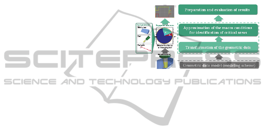
geometrical modelling, Figure 13. Based on the
macroscopic simulation, critical process areas can be
identified or can be investigated for sub-optimal
process performance.
Figure 13: Hierarchical structure of the simulation system
for macroscopic engagement conditions.
Therefore, the toolpath is divided into discrete
segments. At each discrete point on the toolpath, the
contact between the tool and the workpiece
geometry is determined and then used for calculating
the engagement conditions,
Figure
14. Between two
points on the toolpath, the intersection of the
bounding geometry of the tool and the workpiece
model is determined. The set of intersecting points
can be used directly for the calculation of removed
material on the workpiece model. The removed
material data resulting from the tool position and
orientation on the current toolpath point is used to
derive the macro conditions, i.e. the contact angle
ϕ
c
(t,k) and the chip length l
sp
(t,k). At a discrete
instant t of the process, the profile of macroscopic
quantities can be determined along the tool axis by
subdividing the tool in m+1 tool discs, resulting in a
particular value ϕ
c
(t,k) at each tool disc k, where
k=0,1,2,… m.
Since the calculation of macro conditions is
abstracted from the exact cutting geometry, the
computational effort is drastically reduced. So,
macroscopic conditions are calculable throughout
the entire process by avoiding expensive calculation
steps. Both aspects, namely sufficient reliability of
the model as well as demands on efficiency are
achieved. In this regard, efficient techniques for
workpiece update with special consideration of a
sufficiently precise engagement modeling are
indispensable. Especially complex workpiece
ICINCO2013-10thInternationalConferenceonInformaticsinControl,AutomationandRobotics
510
geometries with machining operations consisting of
several 100,000 NC blocks need to be verified in the
macro simulation with the reasonable response
times.
Figure 14: Geometric approach for macroscopic
engagement simulation of multi-axis processes.
3.1 Calculation Models for Macro
Simulation
The calculation of engagement conditions is based
on the geometrical contact of the cutter and the
workpiece. Accurate predictions on the contact
between the tool and workpiece are the basis for
further calculations and therefore essential in the
simulation approach. Both the tool and the
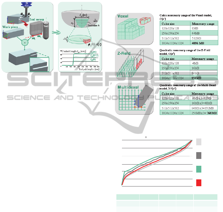
workpiece can be modeled in the context of
geometrical simulation in various ways. Highly
dimensioned and complex workpiece geometries
require a large memory usage and fast methods for
the update during machining. So, the choice of
appropriate “modeling schemes”, i.e. how a
workpiece is discretized, (Stifter, 1995) affects the
simulation accuracy and space complexity greatly,
Figure 15.
A further focus is on the introduction of
modeling schemes with special consideration of a
sufficiently accurate mapping of engagement
conditions since engagement calculations are
directly derived from the discretized elements of the
workpiece model and hence influence the quality of
the simulation results. Practical tests have shown
that the dexel and the multi-dexel scheme provide a
high accuracy for engagement calculation operations
while allowing an efficient dynamic update of the
workpiece, Figure 16.
The workpiece model representation used in this
work is based on the multi-dexel scheme introduced
by Stautner, (Stautner, 2005). Furthermore, the
boundary model of the milling tool, given as a CSG
model, is used to determine the contact area, i.e. the
cutting edges of the tool are neglected. The dexel
scheme is an instance of spatial enumeration
techniques with desired requirements referring
accuracy and performance, (Stifter, 1995).
Figure 15: Space complexity of the modelling schemes
and their memory usage for a cube geometry.
Figure 16: Accuracy of the modelling schemes for
engagement calculation.
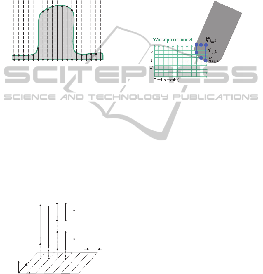
The dexel model of the workpiece is determined
by a set of parallel and equidistant rays intersected
with the original workpiece geometry,
Figure
17. By
intersecting each ray with the workpiece, two points
on a line segment, which is totally inside the
workpiece, are determined. A dexel is defined by
these two points on the line segment. The
intersection points can be calculated with a high
Nominal Δ Z-Fiels Δ Voxel Δ Multidexel
Max. Error
137.54° 10.64° 14.83° 4.23°
Ø Error 0.00° 6.77° 8.23° 2.7°
0
30
60
90
120
Contact angle ϕ
c
[ ]
150
180
Tool path length in y-direction [mm]
50 100 100 150 200
Analytical
Voxel
Z-
Field
Multi dexel
MacroscopicSimulationofMulti-axisMachiningProcesses
511
accuracy since the dexel grid provides float
precision parallel to the ray direction. However, a
single dexel model leads to deviations in
representing the original workpiece if the shape is
sampled parallel to the projection plane of the dexel
grid. Here, the determination of intersection is
depending on the grid interval.
Figure 17: Dexel based representation of the workpiece.
To overcome this insufficiency, the multi-dexel
scheme is used which can be regarded as an
extension of the dexel model. As shown in Figure
18, the multi-dexel model consists of three
overlapping orthogonal dexel grids. Compared to the
single direction dexel model, the multi-dexel scheme
expresses a model more precisely since the
computation of each coordinate of an intersection
point can be performed with float precision. The
multi-dexel model is defined as a set of {d
i,j,k
}, by a
constant grid distance δ relative to the origin point
O, (Ren, 2008). Each dexel d
i,j,k
has two nodes ξ
l
i,j,k
and ξ
u
i,j,k
as the lower and the upper bound of the
dexel segments, Figure 18. The space complexity is
estimated by O(N
x
⋅
N
y
+ N
y
⋅
N
z
+ N
x
⋅
N
z
)
⋅
M
d
∈ O(N²),
where N
i
are the cell numbers along principal axes
and M
d
is the maximum number of dexel nodes.
Figure 18: Logical structure of the dexel model,
(Ren, 2008).
To simulate the material removal by machining,
the contact area between the tool and dexels that are
involved in the cutting are calculated at a given
instant. This means a rearranging of the dexel data at
region of tool-workpiece interaction, while the entire
material removal requires a sequential update of the
dexel elements. These steps are repeated at each
discrete point of the machining toolpath until the
machining process is completed, Figure 19.
Figure 19: Intersection of the tool with the workpiece.
3.2 Calculation of Macroscopic
Engagement Conditions
The contact between the tool and the workpiece can
be calculated by the intersection of the tool
boundary geometry and the dexels. This requires
determining the area of the tool that is in contact
with each dexel and then identifying the
corresponding ξ
l
i,j,k
and ξ
u
i,j,k
for each d
i,j,k
involved
during a cut. Hence, let S
Tool
and S
Workpiece
be defined
as the tool domain and the workpiece domain,
respectively. Further, let p=(p
x
,p
y
,p
z
) ∈ S
Tool
be a
discrete point of S
Tool
and q=(q
x
,q
y
,q
z
) ∈ S
Workpiece
be
a point on the workpiece. If the condition
∃ α,β,γ ∈ {i,j,k} with p
α
≤ q
α
, p
β
=q
β
, p
γ
=q
γ
,
(5)
is satisfied at a discrete point in time t, the tool and
the workpiece are considered to be in engagement
and lead to the engagement domain D(t), which is
defined as follows:
D(t) = {(s
l
, s
u
) | s
l
∈³, s
u
∈³},
(6)
where s
l
=(s
l
x
,s
l
y
,s
l
z
) and s
u
=(s
u
x
,s
u
y
,s
u
z
) fulfill (5) for
a q ∈
S
Tool
. The set D(t) consists of point pairs
describing the line segments which are cut by the
tool at t. The corresponding points of the 2-tupels in
D(t) can be expressed as s
l
=(i,j,ξ
l
i,j,k
) and
s
u
=(i,j,ξ
u
i,j,k
), respectively by regarding the
intersection of the cut dexel d
i,j,k
and S
Tool
in the
nodes ξ
l
i,j,k
and ξ
u
i,j,k
,
Figure
20.
ξ
u
i,j,1
ξ
l
i,j,1
d
i,j,1
ξ
u
i,j,1
ξ
l
i,j,0
d
i,j,0
ξ
u
i+1,j,1
d
i+1,j,1
ξ
l
i+1,j,1
z
y
x
O
δ
ICINCO2013-10thInternationalConferenceonInformaticsinControl,AutomationandRobotics
512
Figure 20: Set of the the intersecting dexel segements with
the tool during the engagement.
To express the contact conditions referring to the
cutting area on the tool, each element of D(t) is
transformed into the coordinate system of the tool
TCS, see section 2.4. Thus, the engagement domain
D
TCS
(t) is defined as
D
TCS
(t) = {(ṡ
l
, ṡ
u
) | ṡ
l
=T
⋅
s
l
-v, ṡ
u
=T
⋅
s
u
-v},
(7)
where s
l
∈ D(t), s
u
∈ D(t) and T ∈
3×3
defined as the
basis transformation matrix build up by the three
vectors n, v
f
, b ∈ ³. The vector v ∈
3
describes the
offset between O and O
TCS.
Furthermore, it can be
easily seen that D
TCS
(t) is bounded by the bounding
geometry of the tool, i.e.
∀(ṡ
l,
ṡ
u
) ∈ D
TCS
(t): (ṡ
l,
ṡ
u
) ⊆ S’
Tool
,
(8)
where S’
Tool
:={T
⋅
q – v | q ∈ S
Tool
}. The macroscopic
engagement conditions are derived by using the
engagement domain D
TCS
(t) at each instant t. As
described in section 2.5, the contact conditions may
vary along the tool axis. In order to estimate the
course of engagement conditions depending on the
tool axis, the engagement area is evaluated by
discretizing the tool along its length in m+1 discs,
Figure
21.
Figure 21: Material removal mapped on the discrete tool
disc along the tool axis.
Each disc has a position and an orientation on the
tool that defines the oblique cutting performed by
that disc segment. For a defined tool orientation
n=(n
x
,n
y
,n
z
), the tool discs can be defined as a set of
planes originated in O
TCS:
={E
k
⊂
³| E
k
={p ∈E
k
|n
x
p
x
+n
y
p
y
+n
z
p
z=
k
⋅
Δz}}
(9)
where k=0, 1, 2,…, m. The contact area for each tool
disc E
k
is determined by finding the intersection of a
line segments (ṡ
l
,ṡ
u
) ∈D
TCS
(t) with E
k
. Hence, the
engagement area of E
k
at a discrete instant t can be
described as
D
TCS
(E
k
,t)={p| ∃(ṡ
l
,ṡ
u
) ∈D
TCS
(t): p∈
E
k
∩(ṡ
l
,ṡ
u
)}.
(10)
For each E
k
and (ṡ
l
,ṡ
u
), it is true that ǁE
k
∩(ṡ
l
,ṡ
u
)ǁ = 1,
i.e. E
k
and (ṡ
l
,ṡ
u
) intersect only in p, except (ṡ
l
,ṡ
u
)
completely lies in E
k
. By recalling (6), for every
p ∈ (ṡ
l,
ṡ
u
) it is also true that p ∈S’
Tool
since p lies on
the line segment limited by ṡ
l
and ṡ
u
. It follows that
D
TCS
(E
k
,t) ⊆ S’
Tool
for some E
k
∈ . Looking closer
to D
TCS
(E
k
,t), it can be seen that
∀ p ∈ D
TCS
(E
k
,t): ǁp - O
TCS
ǁ ≤ r(k)
(11)
for r(k) ∈ and k=0,1,…m, i.e. the contact points in
D
TCS
(E
k
,t) are bounded by the corresponding tool
radius at the tool disc E
k
.
Figure 22: Estimation of the minimal and maximal angles
on a tool disc E
k
.
The particular angular engagement area for a
given disc E
k
is given by the minimal angle ϕ
min
(k)
and the exit angle ϕ
max
(k) on E
k
. These two
parameters provide a compact form to describe the
tool-workpiece engagement at a particular region
along the tool axis at the tool length l=(m+1)
⋅
Δz,
Figure
22
Figure
23. The minimal angle ϕ
min
(k) and
MacroscopicSimulationofMulti-axisMachiningProcesses
513
maximal angle ϕ
max
(k) to each respective disc E
k
are
assigned by finding the point with minimal and
maximal coordinates in x-direction on E
k
. Thus, let
p
min
=(p
x
min
,p
y
min
,p
z
min
) be the corresponding point to
the minimal x-value in D
TCS
(E
k
,t) and
p
max
=(p
x
max
,p
y
max
,p
z
max
) the maximal, respectively.
The angular values of ϕ
max
(k) and ϕ
min
(k) are
determined by
:
,for
0
,for
0
(12)
and
:
,for
0
,for
0
(13)
and ϕ
min/max
(k)≔0
for p
y
min/max
=0. In case of
clockwise rotating tool, it is ϕ
st
(k)=ϕ
max
(k) and
ϕ
ex
(k)=ϕ
min
(k). In case of a counterclockwise rotating
tool, ϕ
st
(k) and ϕ
ex
(k)
are swapped. The contact angle
ϕ
c
(k) at E
k
is estimated by ϕ
c
(k):=ϕ
ex
(k)-ϕ
st
(k),
Figure
23.
Figure 23: Calculation of contact angle on a tool disc.
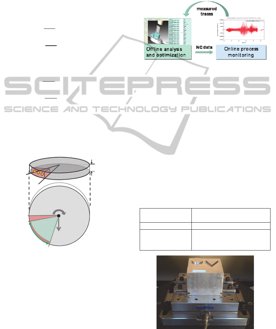
4 RESULTS AND DISCUSSION
The main advantage of process simulation is that
process behaviour can be evaluated before cost
expensive trials are conducted. The link between the
simulation with data from the process monitoring
results in a higher knowledge base about the process
interdependencies in the milling process, Figure 24.
Therefore, a synchronisation between both data
sources has to be developed. As a synchronisation
over time scale is not reliable, because the machine
tool’s acceleration behaviour has to be known
exactly, here an approach using synchronisation over
position is chosen.
Figure 24: Link between offline and online process
analysis.
4.1 Use of the Macro Simulation to
Evaluate Processes
In order to prove the concept of linking simulation
data with process monitoring data, test geometry is
defined and manufactured. The test geometry
consists of simple geometric features. A cuboid, a
cylinder and a triangle are placed on a rectangular
base, Figure 25. As workpiece material Aluminum is
used and the tool is a standard 10 mm diameter shaft
mill with two cutting edges. The workpiece is
mounted on a Kistler 9255B force measurement
platform to acquire the process forces. A Mazak
Variaxis 630-5X II t, which is a 5-axis machining
centre, is used to carry out the experiments.
Table 1: Process setup details and process parameters.
Workpiece
Aluminum
140 mm x 150 mm
Tool 10 mm diameter shaft mill
Cutting parameter
f
z
= 0.1 mm
v
c
= 280 m/min
a
p
= 5 mm
Figure 25: Test setup on Mazak Variaxis 630-5X II t.
Δa
p
N
ϕ
c
(k)
v
f
(t)
ϕ
st
(k)
ϕ
ex
(k)
0
2
ICINCO2013-10thInternationalConferenceonInformaticsinControl,AutomationandRobotics
514
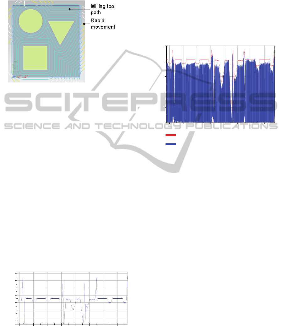
The toolpath and CAM operations are conducted
in the PLM software Siemens NX 8.5. A standard
contour parallel milling strategy is used in
combination with conventional cutting, Figure 26.
Figure 26: Generated toolpath.
A macro simulation of the engagement condition
is carried out and shows the contact angle between
workpiece and tool over time, Figure 27. The macro
conditions were calculated in 3 sec. 430 ms at a
laptop computer (Dell Precision M4600@4x2.2GHz
and 8GB RAM). The toolpath was segmented in
2027 discrete points. The workpiece was discretised
by a precision δ = 0.3mm. From the simulation it can
be seen that the created toolpath leads to frequently
changing engagement situations. As the contact
angle correlates with the process forces the resulting
tool load is varying as well. Critical sections with
high contact angle are identified and can be
optimized through either changing the toolpath or by
reducing the feed rate in the NC program.
Furthermore, sections with rather low contact angles
can be optimized in order to reduce process time. In
addition to optimizing the milling process itself,
process monitoring strategies can be applied.
Integrating and linking geometric information from
macro process simulation with process monitoring
tools opens new ways for online-monitoring of
multi-axis milling processes.
Figure 27: Contact angle over time t.
Using the Kienzle equation, Equation (3), the
expected force depending on the local engagement
situation is calculated. This allows a process
monitoring system to compare online, the expected
force with the current force and decide whether the
milling process is in a stable situation. Compared to
standard monitoring systems no teaching activities
are necessary. The result of calculated monitoring
force and real process force is evaluated in time
domain, Figure 28.
Figure 28: Process monitoring solution for milling
process.
5 CONCLUSIONS AND FURTHER
RESEARCH
Due to frequently changing manufacturing tasks, it
is difficult to control the complexity of machining
processes. However, the parts have to be machined
with high accuracy, robustness and efficiency. Thus,
the shop floors are under strong pressure to deliver
optimal results in shorter times.
In order to efficiently find optimal process
parameters, the level of production automation for
developing processes is important. A simulation
approach that allows the determination and
evaluation of the actual status of the machine and the
process at any time contributes to realize a
systematic optimization of machining operations.
However, complex calculations are used for the
simulation of multi-axis milling processes which are
not yet appropriately controllable despite improved
hardware technologies and parallelization of
algorithms. Important as the use of powerful
hardware and parallel algorithms may be, novel
concepts are needed to minimize the complexity of
the problems to be analysed on the essential level of
120 125 130 135
0
50
100
150
Contact angle / °
Time t / s
120 125 130 135
0
100
200
300
400
500
Active Force F / N
Time t / s
F_calculate
F_measured
MacroscopicSimulationofMulti-axisMachiningProcesses
515

abstraction.
In this paper, the macro simulation for multi-axis
machining processes has been introduced which
focusses on significant parameters in the process. It
enables the reliable detection of disturbances such as
process instabilities or overloads of tool and/or
machine which lead to an excess of tolerances and
hence undesired process deviations. Thus, the
presented work contributes to a significant reduction
of expensive damages and system failures in
production. Apart from the prediction of engagement
conditions, further research is needed to modify
process parameters based on the simulation.
Complex toolpaths in particular can be optimized
regarding the manufacturing and design parameters.
The adjustment of feed rates, the toolpath trajectory
and the tool definition offer a potential for reducing
the process time and creating a more robust
machining process. Hence, future research will focus
on optimizing these parameters based on
macroscopic engagement conditions.
ACKNOWLEDGEMENTS
The authors would like to thank the German
Research Foundation DFG for the support of the
depicted research within the Cluster of Excellence
"Integrative Production Technology for High-Wage
Countries".
REFERENCES
Arntz, K., 2013, Technologie des Mehrachsfräsens von
vergütetem Schnellarbeitsstahl, Aachen
Schug, P. et al, 2012, Durchgängige CAx-Prozessketten,
Forschung an der Werkzeugbau Akademie, Apprimus,
Aachen
Zabel, A., 2010, Prozesssimulation in der Zerspanung,
Vulkan-Verlag, Dortmund
Glaeser, G., 1997, Efficient volume-generation during the
simulation of NC-milling, Proceedings of the
international workshop on visualization and
mathematics’97, pp 89-106 Springer, Heidelberg
Jerard, R., 1989, Approximate methods for simulation and
verification of numerically controlled machining
programs. Visual Computer 5, pp 329-348
Robert, L., 1987, Discrete simulation of NC machining,
Proceedings of the third Annual Symposium on
Computational Geometry, Ontario
Ayasse, J., 2001, Interactive manipulation of voxel
volumes with free-formed voxel tools, VM 2001,
Stuttgart
Stautner, M., 2005, Simulation und Optimierung der
mehrachsigen Fräsbearbeitung, Vulkan Verlag Essen.
CGTech [Online], 2013, http://cgtech.com
Meinecke, M., 2009, Prozessauslegung zum fünfachsigen
zirkularen Schruppfräsen von Titanlegierungen,
Aachen
Diehl A., 2011, Increasing Productivity with Engagement-
Generated Toolpaths, CNC Machining, Vol 14, Iss 47
Klocke F., 2011, Manufacturing Processes 1, Springer,
Berlin,
Ståhl, E., 2012, Metal Cutting. Theories and Models,
Elanders, Lund,
Stifter S., 1995, Simulation of NC Machining Based on
the Dexel Model: A Critical Analysis, Int. Journal for
Advanced Manufacturing Technology, Springer,
London
Ren, Y., 2008, Feature Conservation and Conversion of
Tri-dexel Volumetric Models to Polyhedral Surface
Models for Product Prototyping, Computer-Aided
Design and Application, CAD Solutions,
ICINCO2013-10thInternationalConferenceonInformaticsinControl,AutomationandRobotics
516
