Striving for Better and Earlier Movement Prediction by Postprocessing

of Classiﬁcation Scores

Sirko Straube

, Anett Seeland

and David Feess

2,3

Robotics Group, Faculty of Mathematics and Computer Science, University of Bremen,

Robert-Hooke-Str. 5, 28359 Bremen, Germany

Robotics Innovation Center, German Research Center for Artiﬁcial Intelligence (DFKI GmbH),

Robert-Hooke-Str. 5, 28359 Bremen, Germany

Chair of Global Business, Faculty of Business Administration and Economics, University of Augsburg,

Universitaetsstr. 16, 86159 Augsburg, Germany

Keywords:

EEG, LRP, Brain-computer Interface, Classiﬁcation Score, Movement Prediction, Online Prediction.

Abstract:

Brain-computer interfaces that enable movement prediction are useful for many application ﬁelds from tele-

manipulation to rehabilitation. Current systems still struggle with a level of unreliability that requires im-

provement. Here, we investigate several postprocessing methods that operate on the classiﬁcation outcomes.

In particular, the data was classiﬁed after preprocessing using a support vector machine (SVM). The output

of the SVM, i.e. the raw score values, were postprocessed using previously obtained scores to account for

trends in the classiﬁcation result. The respective methods differ in the way the transformation is performed.

The idea is to use trends, like the rise of the score values approaching an upcoming movement, to yield a

better prediction in terms of detection accuracy and/or an earlier time point. We present results from different

subjects where upcoming voluntary movements of the right arm were predicted using the lateralized readiness

potential from the EEG. The results illustrate that better and earlier predictions are indeed possible with the

suggested methods. However, the best postprocessing method was rather subject-speciﬁc. Depending on the

requirements of the application at hand, postprocessing the classiﬁcation scores as suggested here can be used

to ﬁnd the best compromise between prediction accuracy and time point.

1 INTRODUCTION

Movementprediction using the electroencephalogram

(EEG) has a long standing history in the ﬁeld of

brain-computer interfaces (BCIs) since the discovery

of readiness potentials (Kornhuber and Deecke, 1965;

Libet et al., 1983), which build up long before the ac-

tual movement can occur. Since readiness potentials

reﬂect preparatory activity and movement preparation

can be aborted, these potentials can also disappear af-

ter a short build up without any movement occurring.

However, the closer such a recorded potential gets to

the actual movement, the stronger it is and the less

likely will a prepared movement be cancelled (Fabi-

ani et al., 2007, for a summary). When the move-

ment is ﬁnally executed a corresponding motor po-

tential can be recorded that reﬂects signalling to the

muscles. For movement prediction, different signals

have been applied, from the readiness potential itself

over the lateralized readiness potential (LRP) which is

closer to the movement and cannot easily be aborted

(Blankertz et al., 2006), to speciﬁc frequency compo-

nents in the EEG reﬂecting neural synchronization or

desynchronization (Bai et al., 2011).

Movement prediction can be used as a powerful

tool in various ﬁelds, with the most prominent being

assistance during rehabilitation. Here BCIs predict-

ing a movement can be used to close the gap between

a patient’s intention to move and the actual move-

ment which can result in more intuitive responses

of orthoses (Ahmadian et al., 2013; Kirchner et al.,

2013; Kirchner and Tabie, 2013). Other ﬁelds in-

clude non-medical applications, e.g., during telema-

nipulation of a robotic device the user can be sup-

ported using a movement prediction based on EEG

data (Folgheraiter et al., 2011; Folgheraiter et al.,

2012). The idea is that the human operator experi-

ences a smoother interaction with the telemanipula-

tion device, which knows about an upcoming move-

ment. As in the present study, the movement predic-

tion is often based on the LRP.

Decisions in a movement predicting BCI come

Straube S., Seeland A. and Feess D..

Striving for Better and Earlier Movement Prediction by Postprocessing of Classiﬁcation Scores.

DOI: 10.5220/0004632600130020

In Proceedings of the International Congress on Neurotechnology, Electronics and Informatics (NEUROTECHNIX-2013), pages 13-20

ISBN: 978-989-8565-80-8

 2013 SCITEPRESS (Science and Technology Publications, Lda.)

−4 −3 −2 −1 0

−5

−4

−3

−2

−1

time to movement [s]

classification score

(a)

−4 −3 −2 −1 0

−4

−3

−2

−1

time to movement [s]

classification score

ignore

no mv

(b)

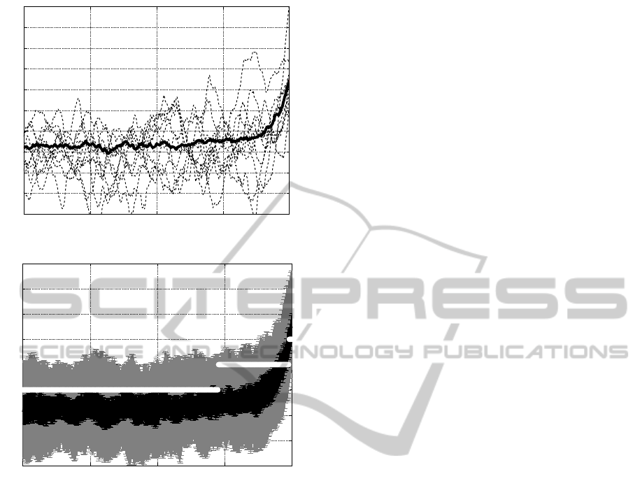
Figure 1: Example data from single subject prior to a move-

ment. Depicted are 4 s of data with the movement onset at

the very right (0ms). (a) The bold black line shows the me-

dian of all 117 epochs. Dashed lines are 10 exemplary sin-

gle trials. (b) Data of the same subject as (a) illustrated as

32/68 percentiles (black) and 5/95 percentiles (dark grey).

The white line denotes time ranges where the data is la-

belled differently for evaluation: no movement (no mv) from

-4000 ms to -1050ms and movement (mv) from -50 ms to

0 ms. In between, data is ignored for true labels (see text).

from some kind of classiﬁer which has to make the

prediction. However, the output of the classiﬁer is

again noisy, so recent approaches try to apply a post-

processing to minimize classiﬁcation errors (Lemm

et al., 2004; Zhu et al., 2006; Solis-Escalante et al.,

2008; Mohammadi et al., 2012). Here, we follow this

rationale by applying simple online-capable functions

to modify the classiﬁer output according to knowl-

edge about its progression. The scenario is the follow-

ing: After processing, the classiﬁer which is a sup-

port vector machine (SVM) assigns a value, the clas-

siﬁcation score, to each data instance (Vapnik, 1995).

The range of these score values depends on the data

at hand and on the classiﬁer and can largely ﬂuctuate

as can be seen in Figure 1. A score of zero denotes

the borderline between the two classes. The ﬁgure il-

lustrates the high ﬂuctuations in single trials and the

consistent trend in the data: When the median score

is considered, the score is constantly staying below

zero, i.e., no movement is classiﬁed, until the scores

rise approximately 500 ms before the movement and

cross zero approximately at 250ms before onset. The

rise in classiﬁcation scores before movement onset

can consistently be observed across subjects. This

means that the rise in score values alone may signal

an upcoming movement so that the progression of the

score values itself can be interpreted as being loosely

correlated to the changes in movement probability.

The question now is whether we can use the

knowledge about this rise in classiﬁcation scores to

make the prediction more stable and/or predict the

upcoming movement earlier. In trying to answer

this question we were seeking for a postprocessing

method that dampens fast ﬂuctuations in classiﬁcation

scores and stabilizes long rises. To this aim, we ap-

plied several methods that modify the current classi-

ﬁcation scores by taking into account previous scores

with a certain weight (see Section 2).

To summarize, if an LRP can be detected by high

levels of the classiﬁcation score, it could potentially

just as well be predicted earlier by detecting the rise

that leads to that elevated level. In the following we

will describe the postprocessing methods that we have

applied. After a description of the experimental data

used, the results will be presented and discussed.

2 POSTPROCESSING METHODS

From the perspective of a movement prediction appli-

cation it is most desirable to perform robust, binary

decisions: A movement will either occur or it will

not. This decision should be made as reliably and

early as possible. From the large margin classiﬁcation

perspective, this means that the classiﬁcation score S

at some point in time t would have to be compared

against some threshold b so that a movement mv is

predicted when

mv iff S

≥ b. (1)

Yet, as illustrated in Figure 1, the score sometimes

suddenly crosses the threshold when the actual move-

ment is still far away, but then only for a short time.

This behaviour hinders reliable prediction when it is

purely based on the raw value of S

crossing b. Look-

ing at the average score progression over time reveals

NEUROTECHNIX2013-InternationalCongressonNeurotechnology,ElectronicsandInformatics

a continuous rise of the score values before the ac-

tual movement. Here, we exploit this systematic be-

haviour to ﬁnd a function F that is able to generate

better movement predictions based on past values of

S, such that

mv iff F(S

t−1

,...,S

t−(k−1)

) ≥ b

(2)

for some speciﬁc threshold b

. k is deﬁned as the

number of scores that are used in F with the current

score being at k = 1. In principle, there are no con-

straints on the functional form of F.

In the present study we apply weights to the cur-

rent and previous k − 1 classiﬁcation outcomes to

transform the current score S

. These weights decay

with the number of steps looked into the past. We

also followed an alternative approach by transform-

ing the current score with the average slope of the

past samples. A detailed description is given in Sub-

section 2.2. Both types of functions (weighting and

slope approach) can be expressed as

F(S

t−1

,...,S

t−(k−1)

) =

+ w

t−1

+ ·· · + w

t−(k−1)

(3)

with some predeﬁned weights w. With this methodol-

ogy we try to boost the score value when previous

scores were similar in value and at the same time

penalize scores when previous ones showed a com-

pletely different trend. The approaches are described

in more detail in the following.

2.1 Fixed Weighting

In this set of functions the weights are generated by

very simple functions, each of which assigns a high

weight to the most current classiﬁcation score sample,

and decreasing weights to older samples.

The functions used are depicted in Fig. 2. All

functions have in common that the weights add up

to one. The coefﬁcients for the

uniform

linear

square

, and

cubic

method are all generated by eval-

uating

∑

i=1

, τ ∈ {1,...,k}, (4)

respectively, with k the number of coefﬁcients used

and the exponent p according to the corresponding

function type. The

exp

coefﬁcients are accordingly

calculated as

expτ

∑

i=1

expi

, τ ∈ {1,...,k}. (5)

Besides these rather universal functions for choos-

ing the weight we added two variants where we ex-

plicitly forced the current value to have a much higher

t t−1 t−2 t−3 t−4 t−5

−0.5

0.5

1.5

score index [classification samples]

weight coefficient

uniform

linear

square

cubic

exp

50+uniform

75+uniform

150+slope

Figure 2: Comparison of the functions used for classiﬁca-

tion score postprocessing using k = 6 coefﬁcients, i.e., the

current score and 5 instances back in time.

weight than the scores corresponding to the previous

instances, since the idea behind the postprocessing

was exactly this: Transform the current score with

its history to weaken fast ﬂuctuations and strengthen

longer trends. Again, the weights were set so that they

add up to one. In the

X+uniform

method, the ﬁrst co-

efﬁcient gets assigned a weight of X%. The remain-

ing weight of [1−(X/100)] is then equally distributed

across the remaining coefﬁcients.

2.2 Slope Approaches

Since the objective is to identify a rise in the classiﬁ-

cation score progression over time we also looked at

modiﬁcations of the score value using local slopes or

averaged slope over the last k samples (i.e., the current

sample and k− 1 instances back in time). Considering

two samples, a local slope ∆S

can be computed as

∆S

− S

t−1

t − (t − 1)

= S

− S

t−1

. (6)

Therefore, the average slope ∆S

k−1

over k samples is

∆S

k−1

(k− 1)

k−1

∑

i=1

t−i+1

− S

t−i

). (7)

which is a telescope sum and boils down to

∆S

k−1

∝ (S

− S

t−(k−1)

). (8)

The corresponding weighting coefﬁcients for this

postprocessing are then

= 1, w

= −1, w

= 0 ∀τ /∈ {1,k},

or w = (1,0,...,0,−1). (9)

In pilot experiments (not shown) this

slope

method was tested and performance levels were con-

sistently far below the performance obtained without

StrivingforBetterandEarlierMovementPredictionbyPostprocessingofClassificationScores

any postprocessing. Due to these performances losses

of at least 0.15 points of balanced accuracy (BA, see

Section 4.1) and in worst cases a performance around

the probability of guessing this method was skipped

for the current study.

Nevertheless, since we were looking for stabiliz-

ing a slope, we chose another promising and simple

variant. Instead of using only the slopes, we modu-

late the current score with the slope approach in a 2:1

fashion (score:slope), so that we obtain a weight vec-

tor w of

w = (1.5,0,...,−0.5). (10)

In other words, in this approach we take the current

score value with 100% and add the slope weighted

with 0.5. This variant is called

150+slope

3 DATA & PREPROCESSING

The data used for evaluation has been described in de-

tail previously (Kirchner and Tabie, 2013; Tabie and

Kirchner, 2013). Originally, muscle activity has been

recorded simultaneously with the EEG. Here, evalua-

tion has been restricted to EEG data.

3.1 Experimental Data

Eight right-handed male subjects (age: 29.9 ± 3.3

years) participated in the study. They gave written

consent to participate and could abort the experiment

at any time. The study was conducted in accordance

with the Declaration of Helsinki. The subjects were

sitting in a comfortable chair in front of a table with

a monitor showing a ﬁxation cross and giving oc-

casional feedback. They executed self-paced, inten-

tional movements with their right arm by releasing

a button and pressing another one situated 30 cm to

the right. A resting period of 5 s between move-

ments had to be performed for a movement to be

counted as valid. Subjects were not informed about

this time constraint, instead negative feedback was

provided (a red circle around the ﬁxation cross) when

they performed a movement too quickly after another.

In each session 120 correctly performed movements

were recorded, divided into 3 runs (40 movements per

run).

3.2 Preprocessing

The EEG was acquired with 5 kHz, ﬁltered between

0.1 Hz to 1 kHz using the BrainAmp DC ampliﬁer

[Brain Products GmbH, Munich, Germany]. Record-

ings were performed using a 128-channel (extended

10-20) actiCap system (reference at FCz). Electrodes

I1, OI1h, OI2h and I2 were used for electrooculogra-

phy and thus not placed on the scalp. For detection of

the physical movement onset a motion capturing sys-

tem consisting of 3 cameras (ProReﬂex 1000; Qual-

isys AB, Gothenburg, Sweden) was used at 500Hz.

After synchronization of the two data streams, the

movement onsets were marked in the EEG.

Preprocessing was performed on overlapping win-

dows of 1 s length cut every 10 ms in a range from

−4000ms to 0ms before a movement. Consequently,

a total of 401 score values were computed per exe-

cuted movement. Data were standardized channel-

wise (subtraction of mean and division by standard

deviation) and decimated to 20Hz. Next, a FFT band-

pass ﬁlter with a pass band of 0.1 to 4Hz was applied.

Since the prediction should be based on the most re-

cent data, we proceeded with the last 200ms of each

window that were processed by an xDAWN spatial

ﬁlter (Rivet et al., 2009) with 4 channels retained. For

feature extraction, raw voltage values were used, stan-

dardized (mean zero, variance one) and classiﬁed by

a SVM (Chang and Lin, 2011) with linear kernel.

For trainable components in the signal process-

ing chain (xDAWN, feature normalization and SVM)

windows ending at −100 and 0 ms were labeled as

movement. Training windows for no movement origi-

nated from non-overlappingwindows (1 s length) that

were continuously cut from the data stream, if no

movement occurred 1 s before and 2s after this win-

dow. In addition, a parameter optimization for the

complexity parameter of the SVM was performed us-

ing a grid search (tested values: 10

,10

−1

,...,10

−6

A 3-fold cross-validation, one fold corresponding

to one experimental run, was applied and classiﬁer

scores were stored for both, training and test data.

4 EVALUATION

As the aim is to detect movements more accurately

and/or earlier, there are basically two criteria for a

good postprocessing. One is the detection accuracy,

the other the time point of detection. Both are consid-

ered for evaluation.

4.1 Movement Detection Accuracy

The prediction of unique events comes along with un-

balanced proportions of the two classes no movement

and movement, i.e., class instances of data containing

the LRP (in our case) will be underrepresented. The

evaluation of the movement detection accuracy has to

take this into account. Thus, the simple accuracy is

misleading (Kubat et al., 1998, for discussion), so a

NEUROTECHNIX2013-InternationalCongressonNeurotechnology,ElectronicsandInformatics

metric is required which is insensitive to imbalanced

classes.

One of the most intuitive measures existing in

such a case is the balanced accuracy (BA) which is

deﬁned as the mean of true positive rate (TPR) and

true negative rate (TNR):

BA =

TPR+ TNR

. (11)

One of the challenges here is to deﬁne a ground truth

of when the relevant signal (i.e., the LRP) is actu-

ally present in the data. While we can postulate that

there must be an LRP prior to each movement, we

still do not know the precise onset of this signal. To

cope with this issue and thereby get unambiguously

labelled data for evaluation, we split the time before a

movement into three phases (compare Figure 1), a no

movement phase from -4000ms to -1050ms, a move-

ment phase from -50ms to 0 ms, and the phase in be-

tween (-1050ms to -50 ms) where the data is ignored

and not labelled at all. With this approach we obtain

a clear labeling in phases where we are sure that the

relevant signal is indeed contained in the data. This

signal is, of course, also present in the ignored time

range, but since we do not know the exact onset this

range is skipped. In the actual application where no

data are skipped, a movement is predicted whenever

the classiﬁer score crosses the threshold.

4.2 Time Point of Detection

The onset of the signal related to movement (here, the

LRP) occurs at an unknown point in time before the

actual movement. This transition out of noise is typ-

ical for event-related potentials and it is reﬂected in

the rise of classiﬁcation scores that we intend to sta-

bilize with the postprocessing approaches introduced

here. Concerning the application, i.e., the predic-

tion of an upcoming movement, the exact time point

is of less importance than a reliable and stable pre-

diction by the classiﬁer. For this, it remains to de-

ﬁne when exactly we consider the LRP as detected—

the classiﬁcation score might at any time rise over

a given threshold for a short period of time due to

noise. For the same reason, the score might fall be-

low the threshold for some samples although the LRP

has—supposedly—already been correctly detected.

To make sure that we base our evaluation on a sta-

ble prediction, the LRP onset was deﬁned as the point

in time where the classiﬁcation scores do not drop be-

low the threshold for N predictions. This point was

found by going back in time from the actual move-

ment onset until the ﬁrst time where this criterion was

not met. With this method, the LRP onset used for

evaluation is then deﬁned as the ﬁrst score sample

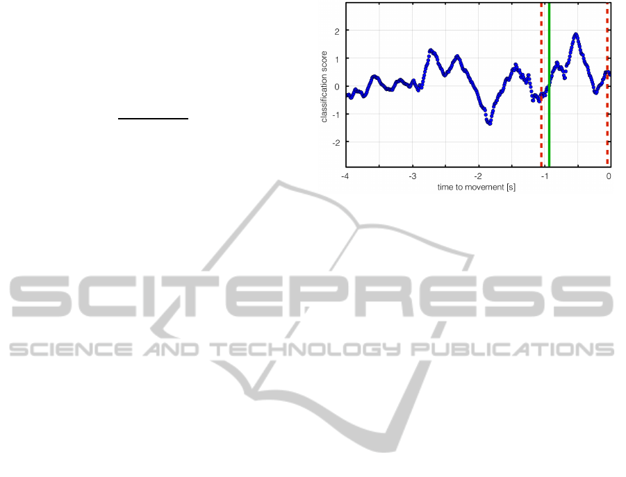
Figure 3: Single trial example for determination of LRP on-

set with N = 10 specifying the number of samples a false

negative classiﬁcation is tolerated. The dashed red lines de-

limit the feasible (transition) area, the solid green line indi-

cates the detected LRP onset. Setting N = 10 provokes that

the small dip around -200ms is ignored.

crossing the threshold after the set of samples staying

below threshold for N predictions.

The choice of N depends on the level of noise,

on the classiﬁcation scores, on the sampling rate, and

on the characteristics of the signal applied for move-

ment prediction. Here, the relevant signal has a length

of approximately 1 s (Fabiani et al., 2007), so we

chose N = 10 as a good compromise between robust-

ness (higher N) and reliability (lower N), i.e., we tol-

erate false classiﬁcations during periods shorter than

100 ms. Increasing the robustness here means to al-

low an earlier estimation of the time point of detec-

tion, because ﬂuctuations in the score progression are

more and more ignored with increasing N. On the

contrary, a decrease of N increases the reliability, be-

cause fewer classiﬁcations of no movement can occur

after the estimated time point of detection, but this

comes at the cost of a higher sensitivity to outliers.

To give an alternative view on the value of N: Setting

N = 10 in our data means that the movement onset is

deﬁned as the ﬁrst score sample crossing the threshold

after a 100 ms window without any predicted move-

ment (viewed backwards from the actual movement

onset). The approach is illustrated in Figure 3.

4.3 Evaluation Procedure

For each subject and cross-validation fold two data

sets exist: one training data set (80 movements) and

one test data set (40 movements). The training set

is the one used to train the classiﬁer producing the

classiﬁcation scores. Due to the fact that the post-

processing methods introduced here change the abso-

lute value of the classiﬁcation score, the score thresh-

olds (transition from one class to the other) were

re-adjusted for each method, respectively, using the

StrivingforBetterandEarlierMovementPredictionbyPostprocessingofClassificationScores

−500 −400 −300 −200 −100 0

0.75

0.8

0.85

0.9

0.95

1.05

relative prediction onset [ms]

relative performance [BA]

uniform

linear

square

cubic

exp

50+uniform

75+uniform

150+slope

(a)

−800 −700 −600 −500 −400 −300 −200 −100 0 100

0.7

0.75

0.8

0.85

0.9

0.95

1.05

relative prediction onset [ms]

relative performance [BA]

(b)

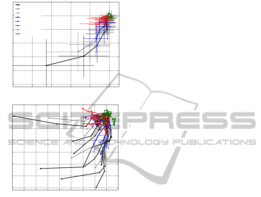
Figure 4: Performance changes (BA and onset time) of post-

processing methods. The results are illustrated relative to

the case where the scores were not further processed, il-

lustrated as a white dot at (0,1). Each data point corre-

sponds to a different k ∈ {1,2, 4,8,12,16,20,40,60,100}

(see text). In (a) the grand average results over all subjects

are shown as mean and standard deviation for each k, re-

spectively. Thus, there is one line for each method applied.

In (b) the same results are shown for all subjects, separately.

training data, before evaluation was performed on the

test data. The results presented in the following show

the performance in terms of detection accuracy and

time point of detection on the test data.

5 RESULTS & DISCUSSION

All investigated methods introduced in Section 2 and

illustrated in Figure 2 were tested for different values

of the parameter k ∈ {1,2,4,8, 12,16,20,40,60, 100}

which is the number of scores used with the respec-

tive method. Since a key motivation for the current

work was to modify the current score by the values

of the neighbouring scores, we chose a ﬁner granular-

ity for sampling near the current score. Without post-

processing, the movements were predicted on average

over all subjects 180 ms before the movement onset

with a balanced accuracy of 0.8. Since we were inter-

ested in performance improvements concerning these

two measures, the results are illustrated as relative

changes according to these reference performances

in Figure 4 (a). The ﬁgure shows the average result

for all methods applied for the two criteria detection

accuracy and time point of detection (see Section 4).

Here each data point corresponds to a particular value

for k, with k = 100 being the ﬁrst data point on the

lower left of the plot and the next smaller value for

k being the next on the connecting line. Finally, all

methods meet at k = 1 on the upper right at a relative

prediction onset of 0 ms and a relative performance of

1, because all of these have an identical weight vector

of w = (1). This point (highlighted as white spot in

Figure 4) with k = 1 is equal to the reference perfor-

mance without any postprocessing.

The results in Figure 4 (a) indicate that the perfor-

mance obtained when using the raw score values was

already on a high level regarding the time point of de-

tection and the classiﬁcation accuracy. In the ﬁgure,

a postprocessing method outperformingthis reference

would be on the upper left relative to this point. This

we observed only for the slope approach

150+slope

where we found conﬁgurations for k ∈ {2,4} that re-

vealed a slight improvement on average in both, ac-

curacy and time point.

From the ﬁgure, it is far more apparent that most

methods enabled an earlier prediction of the move-

ment on the cost of (mostly) slight performancedrops.

In the most extreme case for the

uniform

approach

with k = 100, this means more than 300 ms ear-

lier prediction at a loss of 18% of the initial perfor-

mance. Overall improvements in classiﬁcation accu-

racy on the average level were only revealed for the

150+slope

approach.

The reason for the large standard deviations de-

picted in Figure 4 (a) is disclosed by illustration of

the single-subject results in Figure 4 (b). The beneﬁt

of the applied method strongly differed between sub-

jects, so that the results in Figure 4 (a) only show the

rough trend. On the single-subject level we observed

slight improvements for both, time point and accu-

racy. However, the best method was subject-speciﬁc.

Again, most extreme differences where achieved us-

ing the

uniform

approach: Using k = 100 we could

detect the movement nearly 800 ms earlier without

any performance loss for one subject, while the same

conﬁguration resulted in only 100 ms earlier detec-

tion at a loss of 30% of the initial performance for an-

NEUROTECHNIX2013-InternationalCongressonNeurotechnology,ElectronicsandInformatics

other. In the analysis, especially subjects with a worse

performance on the raw scores could beneﬁt from the

postprocessing.

To summarize, the postprocessing methods pre-

sented here provide a tool to modify mainly the earli-

ness of the prediction and to a little extent the clas-

siﬁcation accuracy. The

150+slope

method with

k ∈ {2,4} worked best on the average level and en-

hanced both, time point of detection and accuracy. On

the single-subject level, the individual best method

differed, so that the spectrum presented here can serve

as a general framework to adjust the movement pre-

diction according to the respective application and/or

the data of the individual subject.

6 CONCLUSIONS

Without any postprocessing, the classiﬁcation of each

window is performed independentlyof the neighbour-

ing windows. However, we can see in the distribu-

tions of these classiﬁcation outcomes that they intrin-

sically carry information about the probability of an

upcoming event, like the rise in scores illustrated in

Figure 1. Here, we use simple methods that can eas-

ily be applied during online movement prediction to

make use of this knowledgeand stabilize a single clas-

siﬁcation by the surrounding ones. The methodology

introduced here can be used as a tool to improve clas-

siﬁcation outcomes.

Since the performance and the time point of pre-

diction can be both equally relevant for an application,

we considered these two measures together. Taking

these, we could show that the applied methods suc-

ceed for individual subjects in improving the accuracy

and/or time point of prediction, although we could not

ﬁnd one straightforward solution in the current study

for all subjects investigated. For most methods we

found a trade-off between these two metrics. This

means for the application of such a movement predict-

ing system, that one can indeed enhance the system,

but has to carefully chose the postprocessing method

according to the requirements of the intended appli-

cation.

On average we could observe an improvement of

both, time point of detection and accuracy, using the

150+slope

method with small values of k. However,

we found the most pronounced effects on the single-

subject level: the proposed methods performed in-

dividually different. In an application, such a high

subject-speciﬁcity can be dealt with using two ap-

proaches: either extra calibration time is used to ﬁnd

the best individual method, or the prediction itself is

integrated in the application in a way that is ﬂexible

or robust enough to make use of the possible beneﬁts

illustrated here. Since the predictions obtained with-

out postprocessing can serve as a reliable fallback op-

tion, this could be realized, e.g., by using a number

of the proposed approaches on top and making the ﬁ-

nal prediction from the ensemble. More in general,

although the ﬁnding of a subject speciﬁcity is consis-

tent with results from other postprocessing methods

(Mohammadi et al., 2012), it should be helpful to re-

veal the particular origins of these effects in the score

progression to develop a method that generalizes bet-

ter. So far, existing postprocessing methods operate

rather blindly on the data which may cause the indi-

vidual differences.

While most research is dedicated to improvement

of the classiﬁer and/or preprocessing algorithms, the

idea of postprocessing of classiﬁcation outcomes as

such is not completely new. Techniques for incorpo-

rating preceding probabilities to enhance the current

prediction have been proposed (Lemm et al., 2004;

Zhu et al., 2006), but not been evaluated in the way

we did in the present study. Therefore and since SVM

scores do not directly represent probabilities like in

a Bayesian framework, a direct comparison with the

methods we proposed is difﬁcult. However, from the

technical point of view all of these methods have in

common that they actually manipulate single predic-

tion outcomes making use of the individual predic-

tion history. Other techniques exist for postprocessing

that rather operate on the global level by changing the

decision criterion of the classiﬁer or using additional

thresholds. Here, threshold selection, dwell time op-

timization or debiasing of the score time course have

been proposed (Solis-Escalante et al., 2008; Moham-

madi et al., 2012). Due to their different nature, these

techniques can be easily combined with what we pro-

posed here, as we already implicitly did by including

threshold optimization (see Section 4.3) and selecting

a stability criterion of 100 ms (N = 10; see Section

4.2 and Figure 3), which can be interpreted as a dwell

time.

With the approach outlined here, other and more

complex algorithms can of course be used, although

they might have the possible drawback of being too

computationally complex for an online predicting

system. Generally, the methods applied here are not

speciﬁc for the context of movement prediction, so

they can be used in any context where such postpro-

cessing may be helpful.

ACKNOWLEDGEMENTS

This work was supported by the German Bundesmin-

StrivingforBetterandEarlierMovementPredictionbyPostprocessingofClassificationScores

isterium fur Wirtschaft und Technologie (BMWi,

grant FKZ 50 RA 1012 and grant FKZ 50 RA 1011).

The authors like to thank Marc Tabie for providing us

with the evaluation data.

REFERENCES

Ahmadian, P., Cagnoni, S., and Ascari, L. (2013). How ca-

pable is non-invasive EEG data of predicting the next

movement? A mini review. Frontiers in Human Neu-

roscience, 7:124.

Bai, O., Rathi, V., Lin, P., Huang, D., Battapady, H., Fei,

D.-Y., Schneider, L., Houdayer, E., Chen, X., and

Hallett, M. (2011). Prediction of human voluntary

movement before it occurs. Clinical Neurophysiology,

122(2):364–372.

Blankertz, B., Dornhege, G., Lemm, S., Krauledat, M., Cu-

rio, G., and M¨uller, K. (2006). The Berlin Brain-

Computer Interface: machine learning based detec-

tion of user speciﬁc brain states. Journal of Universal

Computer Science, 12(6):581–607.

Chang, C.-C. and Lin, C.-J. (2011). LIBSVM:

A library for support vector machines. ACM

Transactions on Intelligent Systems and Tech-

nology, 2:27:1–27:27. Software available at

http://www.csie.ntu.edu.tw/ cjlin/libsvm.

Fabiani, M., Gratton, G., and Federmeier, K. D. (2007).

Event-related brain potentials: Methods, theory, and

applications. In Cacioppo, J., Tassinary, L. G., and

Berntson, G. G., editors, Handbook of Psychophys-

iology, pages 85–119. Cambridege University Press,

Cambridge [u.a], 3rd edition.

Folgheraiter, M., Jordan, M., Straube, S., Seeland, A., Kim,

S. K., and Kirchner, E. A. (2012). Measuring the im-

provement of the interaction comfort of a wearable ex-

oskeleton. International Journal of Social Robotics,

4(3):285–302.

Folgheraiter, M., Kirchner, E. A., Seeland, A., Kim, S. K.,

Jordan, M., W¨ohrle, H., Bongardt, B., Schmidt, S.,

Albiez, J., and Kirchner, F. (2011). A multimodal

brain-arm interface for operation of complex robotic

systems and upper limb motor recovery. In Vieira,

P., Fred, A., Filipe, J., and Gamboa, H., editors, In

Proceedings of the 4th International Conference on

Biomedical Electronics and Devices (BIODEVICES-

11), pages 150–162, Rome. SciTePress.

Kirchner, E. A., Albiez, J., Seeland, A., Jordan, M., and

Kirchner, F. (2013). Towards assistive robotics for

home rehabilitation. In Chimeno, M. F., Sol´e-Casals,

J., Fred, A., and Gamboa, H., editors, In Proceedings

of the 6th International Conference on Biomedical

Electronics and Devices (BIODEVICES-13), pages

168–177, Barcelona. SciTePress.

Kirchner, E. A. and Tabie, M. (2013). Closing the gap:

combined EEG and EMG analysis for early movement

prediction in exoskeleton based rehabilitation. In Pro-

ceedings of the 4th European Conference on Techni-

cally Assisted Rehabilitation - TAR 2013.

Kornhuber, H. H. and Deecke, L. (1965). Hirnpoten-

tial¨anderungen bei Willk¨urbewegungen und passiven

Bewegungen des Menschen: Bereitschaftspotential

und reafferente Potentiale. Pﬂ¨uger’s Archiv f¨ur die

gesamte Physiologie des Menschen und der Tiere,

284(1):1–17.

Kubat, M., Holte, R. C., and Matwin, S. (1998). Machine

learning for the detection of oil spills in satellite radar

images. Machine Learning, 30(2-3):195–215.

Lemm, S., Sch¨afer, C., and Curio, G. (2004). BCI competi-

tion 2003–data set III: probabilistic modeling of sen-

sorimotor mu rhythms for classiﬁcation of imaginary

hand movements. IEEE Transactions on Biomedical

Engineering, 51(6):1077–80.

Libet, B., Gleason, C. A., Wright, E. W., and Pearl, D. K.

(1983). Time of conscious intention to act in relation

to onset of cerebral activity (readiness-potential) the

unconscious initiation of a freely voluntary act. Brain,

106(3):623–642.

Mohammadi, R., Mahloojifar, A., and Coyle, D. (2012).

A combination of pre- and postprocessing techniques

to enhance self-paced BCIs. Advances in Human-

Computer Interaction, 2012:3:1–3:10.

Rivet, B., Souloumiac, A., Attina, V., and Gibert, G. (2009).

xDAWN algorithm to enhance evoked potentials: ap-

plication to brain-computer interface. IEEE Transac-

tions on Biomedical Engineering, 56(8):2035–2043.

Solis-Escalante, T., M¨uller-Putz, G., and Pfurtscheller, G.

(2008). Overt foot movement detection in one single

laplacian EEG derivation. Journal of Neuroscience

Methods, 175(1):148–153.

Tabie, M. and Kirchner, E. A. (2013). EMG onset detec-

tion – comparison of different methods for a move-

ment prediction task based on EMG. In Alvarez,

S., Sol´e-Casals, J., Fred, A., and Gamboa, H., ed-

itors, In Proceedings of the 6th International Con-

ference on Bio-inspired Systems and Signal Process-

ing (BIOSIGNALS-13), pages 242–247, Barcelona.

SciTePress.

Vapnik, V. N. (1995). The nature of statistical learning the-

ory. Springer New York, Inc., New York, NY, USA.

Zhu, X., Wu, J., Cheng, Y., and Wang, Y. (2006). GMM-

based classiﬁcation method for continuous prediction

in brain-computer interface. In Proceedings of the

18th International Conference on Pattern Recognition

- Volume 01, ICPR ’06, pages 1171–1174, Washing-

ton, DC, USA. IEEE Computer Society.

NEUROTECHNIX2013-InternationalCongressonNeurotechnology,ElectronicsandInformatics