
Natural Handling of Uncertainties in Fuzzy Climate Models
Carlos Gay García
and Oscar Sánchez Meneses
Centro de Ciencias de la Atmósfera, Universidad Nacional Autónoma de México,
Ciudad Universitaria, Mexico. D.F., Mexico
Keywords: Uncertainty, Greenhouse Gas Emissions, Climate Sensitivity, General Circulation Models.
Abstract: The wide range of the IPCC emission scenarios and the corresponding concentrations, forcings and
temperature obtained with the use of the Magicc/Scengen Model are substituted by linearly increasing
emissions that preserve the ranges of the values for the concentrations forcings and temperatures. In fact
IPCC values are comprised within the values of the linear emissions. These allow the identification of
simple relationships that are translated to fuzzy rules that in turn conform the fuzzy model. The sources of
uncertainty that the model permits to explore are: the uncertainty due to not knowing what the emissions are
going to be in the future, the one related to the climate sensitivity of the models (this has to do with different
parameterizations of processes used in the models) and the uncertainties in the temperature maps produced
by the models. Here we produce maps corresponding to 1, 2, 3, etc., degrees centigrade of temperature
increase and discuss the timing of exceeding them. Therefore the argument instead of talking about the
uncertainty in temperature at a certain date becomes about the uncertainty in the date certain temperature
will be reached. The timing becomes another uncertainty.
1 INTRODUCTION
In a recent publication, Gay et al. (2012) simplified
the emission scenarios developed by the
Intergovernmental Panel on Climate Change (IPCC)
using linear functions of time that after being fed to
the Magicc model (Wigley, 2008), produced the
same wide range of concentrations of greenhouse
gases (GHG) and aerosols, and the corresponding
range of temperatures in 2100. These results show
very clearly that higher temperature increases
correspond to higher emission of GHG and higher
atmospheric concentrations. This fact can be
transformed into linguistic rules that in turn are used
to build a fuzzy model, which uses concentration
values of GHG as input variables and gives, as
output, the temperature increase projected for year
2100. Based on the same principles a second fuzzy
model is presented that includes a second source of
uncertainty: climate sensitivity.
It is our intention to extend these results and
produce maps of temperature.
It has been customary to ask what the
temperature is going to be in 2030 or in 2050 and
proceed to estimate the impacts that the changed
temperature would have on social or economic
sectors and activities that either may improve or
most probably would be affected in a negative way.
But in 2030 or in 2050 different models say different
things so, what do we do? Use ensembles? Use the
averages? Consider the standard deviation? Is the
physics consistent? Here we propose to show
temperature maps corresponding to global increases
of 1, 2, 3, etc., degrees centigrade, give an idea of
the uncertainty in timing, in contrast to the
uncertainty in temperature for a certain date. This
means that depending on the emissions,
concentrations etc., the larger these variables, the
sooner 1, 2, etc., degrees will be reached and
considering other sources of uncertainty like the
sensitivity, the pace of change may increase
considerably. When we display the information in
two dimensions produced by different models then
the uncertainty due to different modeling strategies
has to be considered.
We think that it is easier to consider a degree by
degree strategy than one based on dates. The
question of what to do if the temperature increases
one degree or what should we be doing right now
because the temperature is reaching one degree by
2021 (in the worst of cases) and if we do nothing we
will be two degrees warmer by 2039 with grave
consequences for all.
537
Gay García C. and Sánchez Meneses O..
Natural Handling of Uncertainties in Fuzzy Climate Models.
DOI: 10.5220/0004633605370544
In Proceedings of the 3rd International Conference on Simulation and Modeling Methodologies, Technologies and Applications (MSCCEC-2013), pages
537-544
ISBN: 978-989-8565-69-3
Copyright
c
2013 SCITEPRESS (Science and Technology Publications, Lda.)
2 METHOD
By using linear and non-intersecting emission
trajectories, concentrations of GHG and global mean
temperatures increases can be directly related as
illustrated in figures 1 and 2 of Gay et al. (2012).
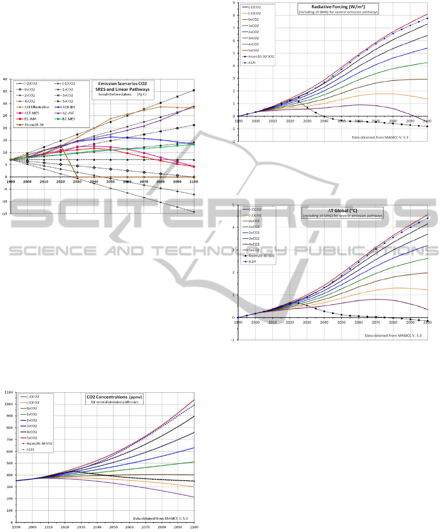
Figure 1: Emissions scenarios CO2, Illustrative SRES
(Nakicenovic, et al. 2000) and Linear Pathways. (-2) CO2
means -2 times the emission (fossil + deforestation) of
CO2 of 1990 by 2100 and so for -1, 0, 1, to 5 CO2. All the
linear pathways contain the emission of non CO2 GHG as
those of the A1FI. 4scen20-30 scenario follows the
pathway of 4xCO2 but at 2030 all gases drop to 0
emissions or minimum value in CH4, N2O and SO2 cases.
With the linear emission pathways shown in the
previous figure, used as input for the Magicc model,
Gay et al. (2012) calculated the resulting
concentrations (figure 2); radiative forcings (figure
3) and global mean temperature increments (figure
4) that we repeat here for clarity.
Figure 2: CO2 Concentrations for linear emission
pathways (4scen20-30 SO2 and A1FI are shown for
reference). Data calculated using Magicc V. 5.3.
We would like to remark a statement made before
(that can be directly observed in Fig. 4): if we want
to keep temperatures at two degrees or less by the
Figure 3: Radiative forcings (all GHG included) for linear
emission pathways and A1FI SRES illustrative, the
4scen20-30 SO2 only include SO2. Data calculated using
Magicc V. 5.3.
Figure 4: Global mean temperature increments for linear
emission pathways, 4scen20-30 SO2 and A1FI; as
calculated using Magicc V. 5.3.
year 2100, we should have concentrations in 2100
consistent with the -2CO2, -1CO2 and 0CO2
trajectories. The latter is a trajectory of constant
emissions equal to the emissions in 1990 that gives
us a temperature of two degrees by year 2100.
From the linear representation, it is easily
deduced (as mentioned earlier) that very high
emissions correspond to very large concentrations,
large radiative forcings and large increases of
temperature.
These simple observations are basic for the
formulation of the fuzzy model, based on linguistic
rules of the IF-THEN form, capable of estimating
increases of temperature. The fuzzy model was built
using the results of the Magicc model (Wigley,
2008) as crisp mathematical model, and Zadeh´s
extension principle (Zadeh, 1965).
For illustrative purposes (the full rules are
reported in Gay et al., 2013) we repeat here the first
two rules of the 18 that were developed previously:
SIMULTECH2013-3rdInternationalConferenceonSimulationandModelingMethodologies,Technologiesand
Applications
538
1. If (concentration is (-2)CO2) and
(sensitivity is low) then (deltaT is
T1) (1)
2. If (concentration is (-1)CO2) and
(sensitivity is low) then (deltaT is
T2) (1)
…
where the triangular fuzzy sets corresponding to T1
and T2 are (0.07, 0.07, 1.23) and (0.07, 0.61, 1.98)
respectively.
The 18 rules were obtained from the combination
of 6 concentrations, projected to 2100 and consistent
with 6 linear emission trajectories, and 3 fuzzy
values for the sensitivity of climate which are 1.5,
3.0 and 6.0 deg C/W/m2, all the values were taken
from the data previously generated by successive
runs of Magicc software.
Once we have the global temperatures and an
idea of the associated uncertainty due to different
emission paths and sensitivities we would like to
convert this information to a two dimensional
display of temperatures. The way to accomplish this
is using the same idea for scaling employed in the
Magicc/Scengen system (Wigley, 2008). This
consists of scaling the value that results from
running for a Global Circulation model (GCM)
option (one of 20 possible), for example with double
CO2 at a certain grid point in the following way:
T
new
= T
grid
/T
map
x T
magicc
(1)
where T
new
is the scaled temperature, T
grid
is the
value of the temperature given by the GCM at a
certain position, T
map
is the average temperature
(global) of the map and T
magicc
is the temperature
given by the simple model
However, emissions and sensitivity introduce
uncertainties in the temperature that in turn must be
reflected in the scaled temperature.
If we denote the uncertainty by a then we
propose:
T
new
= T
grid
/T
map
x T
magicc
(2)
where T
magicc
, is in fact a fuzzy number and
consequently T
new
new also is.
We have to mention that another source of
uncertainty is which GCM we use. We will try to
illustrate this point too.
From the application of the Magicc/Scengen to
the emission trajectories developed in the previous
paper (Gay et al., 2012) we can extract the years in
which the 1, 2, 3 and 4 degrees centigrade thresholds
are reached.
According to the IPCCs Fourth Assessment
Report (IPCC-WGI, 2007) the best estimate for the
sensitivity is 3.0 however this parameter varies from
1.5 to 6, as mentioned before, so there is a source of
uncertainty associated with this parameter. This is
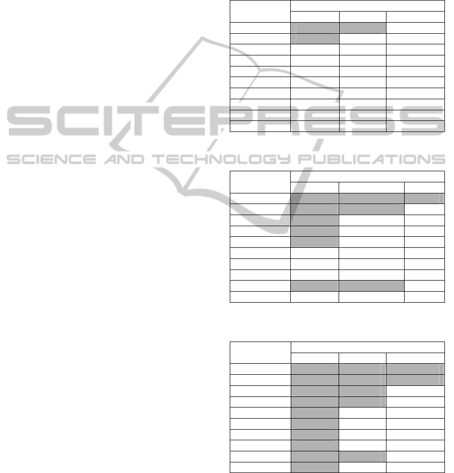
shown by the different values in the tables 1 to 5.
Dates for emission scenarios B1-IMA and A1FI-MI
(Nakicenovic et al. 2000) are shown for reference.
Table 1: Dates to achieve the 1 °C thresholds following
linear emission trajectories from -2CO2 to 5CO2.
Emission
Trajectory
Sensitivity (deg C/W/m2)
1.5 3.0 6.0
-2CO2 2049
-1CO2 2057 2039
0CO2 2079 2048 2033
1CO2 2063 2042 2029
2CO2 2056 2038 2027
3CO2 2051 2035 2024
4CO2 2047 2032 2023
5CO2 2044 2030 2021
B1-IMA 2090 2043 2027
A1FI-MI 2046 2033 2024
Table 2: Dates to achieve the 2 °C thresholds following
linear emission trajectories from -2CO2 to 5CO2.
Emission
Trajectory
Sensitivity (deg C/W/m2)
1.5 3.0 6.0
-2CO2
-1CO2 2073
0CO2 2100 (1.98°C) 2059
1CO2 2072 2052
2CO2 2064 2048
3CO2 2093 2058 2045
4CO2 2081 2054 2042
5CO2 2053 2051 2039
B1-IMA 2057
A1FI-MI 2076 2053 2042
Table 3: Dates to achieve the 3 °C thresholds following
linear emission trajectories from -2CO2 to 5CO2.
Emission
Trajectory
Sensitivity (deg C/W/m2)
1.5 3.0 6.0
-2CO2
-1CO2
0CO2 2087
1CO2 2071
2CO2 2093 2064
3CO2 2081 2059
4CO2 2074 2055
5CO2 2069 2052
B1-IMA 2095
A1FI-MI 2070 2054
Taking into account the opinion of the IPCC that the
best estimate for the sensitivity is 3, it can be said
that we would be exceeding the one degree threshold
by 2030 (sensitivity of 3 and emission trajectory
of 5CO2). However due to the values that this
NaturalHandlingofUncertaintiesinFuzzyClimateModels
539
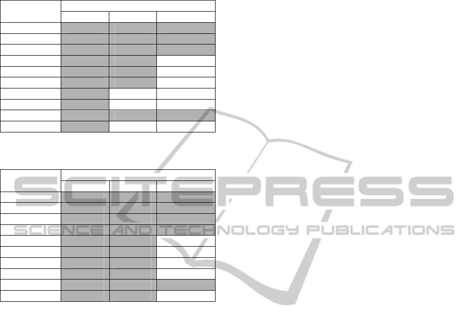
Table 4: Dates to achieve the 4 °C thresholds following
linear emission trajectories from -2CO2 to 5CO2.
Emission
Trajectory
Sensitivity (deg C/W/m2)
1.5 3.0 6.0
-2CO2
-1CO2
0CO2
1CO2 2095
2CO2 2080
3CO2 2073
4CO2 2097 2068
5CO2 2088 2064
B1-IMA
A1FI-MI 2090 2065
Table 5: Dates to achieve the 5 °C thresholds following
linear emission trajectories from -2CO2 to 5CO2.
Emission
Trajectory
Sensitivity (deg C/W/m2)
1.5 3.0 6.0
-2CO2
-1CO2
0CO2
1CO2
2CO2 2100
3CO2 2088
4CO2 2080
5CO2 2075
B1-IMA
A1FI-MI 2077
parameter may assume (1.5 to 6) this threshold may
be delayed to 2044 if the sensitivity is 1.5 or may be
advanced to 2021 if the sensitivity is 6. These values
for the threshold correspond to our worst emissions
scenario 5CO2. If we continue mounted in the same
scenario we could be reaching 6 °C by 2087 and
almost 7 °C by 2100.
Again for the 3 °C threshold we could be
surpassing it as early as 2052 and the “best estimate”
would be 2069; if the sensitivity were 1.5 the 3 °C
temperature would not be reached.
From these tables we can also learn that if the
sensitivity is 6 there is no way of staying at two
degrees unless the concentrations of CO2 had
followed the -2CO2 trajectory: negative emissions
that means very strong subtraction of CO2 from the
atmosphere.
If we were lucky and the climate sensitivity had
a value of three the concentration would have to be
equivalent to the 0CO2 path in 2100 this is about
300 ppmv.
There are obvious messages from the tables: the
smaller the emissions the later the thresholds are
exceeded, if we want small increases of temperature
then we need to impose small emissions or more
precisely small concentrations of CO2.
Two sources of uncertainty are illustrated in the
tables, the first coming from the emissions: large
emissions large temperature changes and the second
due to our imprecise knowledge of the climate
sensitivity of the models. One uncertainty is for the
politicians because emissions depend on policy and
the second for the scientists who may narrow the gap
in the estimations of climate sensitivity.
3 RESULTS
The results of the fuzzy model that combines six
levels of concentrations of CO2, from -2CO2 to
3CO2 in year 2100 (where 1CO2 identifies the
concentration associated to the emissions in 1990),
and 3 levels of sensitivity: 1.5, 3 and 6 are presented
here. The model, that incorporates the uncertainties
mentioned above, consisting of 18 fuzzy rules (Gay
et al., 2013), is run to obtain global temperatures
increases in year 2100 and their corresponding
uncertainty intervals. This information is then used
to produce two-dimensional maps depicting
physically consistent geographical distributions of
temperatures which in turn are consistent with global
temperatures obtained from our fuzzy model. That
the temperatures are physically consistent can be
justified by using the results of a physically
consistent model, in the same way the
Magicc/Scengen does: using the results of runs of
different GCMs.
The fuzzy model with the best estimate for the
sensitivity is used to get the uncertainty intervals for
1, 2, 3 and 4 °C.
In the fuzzy model the value of the sensitivity is
fixed at the best estimate of 3 and varying the
concentration we try to get 1, 2, 3, etc degrees. The
temperature is a function of the concentration. In this
way we obtain:
For an increase of one degree the concentration
of CO2 required is 220 ppmv and the uncertainty
interval is from 0.08 to 2.17 degrees, based on the
fuzzy sets feet presented in Gay et al. (2013) and
reproduced here as a graph (see figure 5). Therefore
for a one degree global increase the uncertainty
extends to more than two degrees, consequently for
a 1 °C global increase, maps for one and two degrees
(see ahead,
figure 7) are to be considered.
If T is 2 degrees the interval is from 0.08 to
3.27 °C; for 3 and 4 degrees the uncertainty intervals
are from 1.07 to 5.02 °C and from 1.82 to 6.41 °C
respectively (
see figure 6). Therefore for a 3 °C
global increase the uncertainty extends to 5 °C so,
maps corresponding to 3, 4 and 5 degrees should be
considered.
SIMULTECH2013-3rdInternationalConferenceonSimulationandModelingMethodologies,Technologiesand
Applications
540
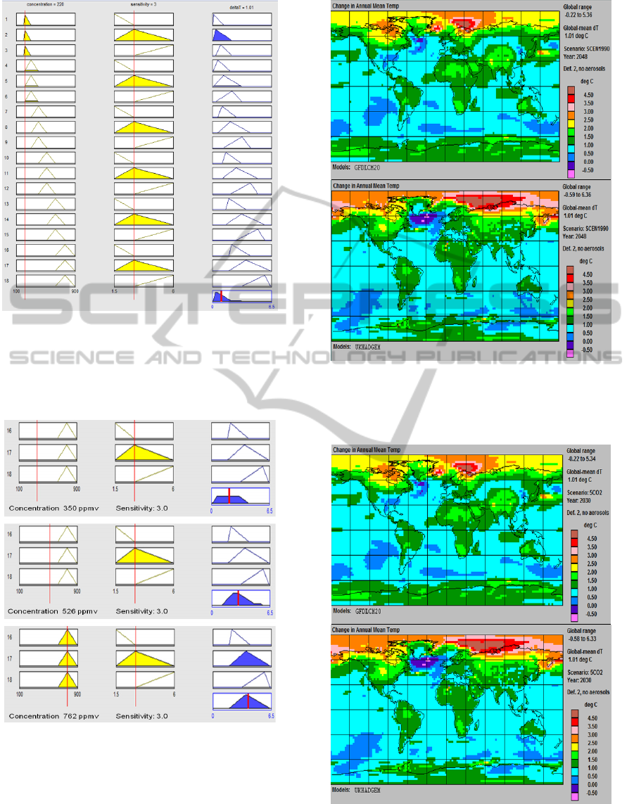
Figure 5: The 18 rules of the fuzzy model for the
estimation of global mean temperature increase T, for a
concentration of CO2 of 220 ppmv and sensitivity of 3.0
deg C/W/m2. The uncertainty interval is (0.08, 2.17) or
(0.08, 3.27) deg C considering the elongated part
(calculated with MATLAB).
Figure 6: Similar to figure 5, estimation of global mean
temperature increase T and its uncertainty intervals
(from the feet of the triangular fuzzy sets) for
concentrations of CO2 of: 350 ppmv (upper panel) with
2.01 °C (0.08 to 3.27); 526 ppmv (middle panel) with 3 °C
(1.07 to 5.02) or (1.07 to 5.75) considering the elongated
part and 762 ppmv (lower panel) with 3.98 °C (1.82 to
6.41). Data calculated with MATLAB only the last 3 are
shown for simplicity.
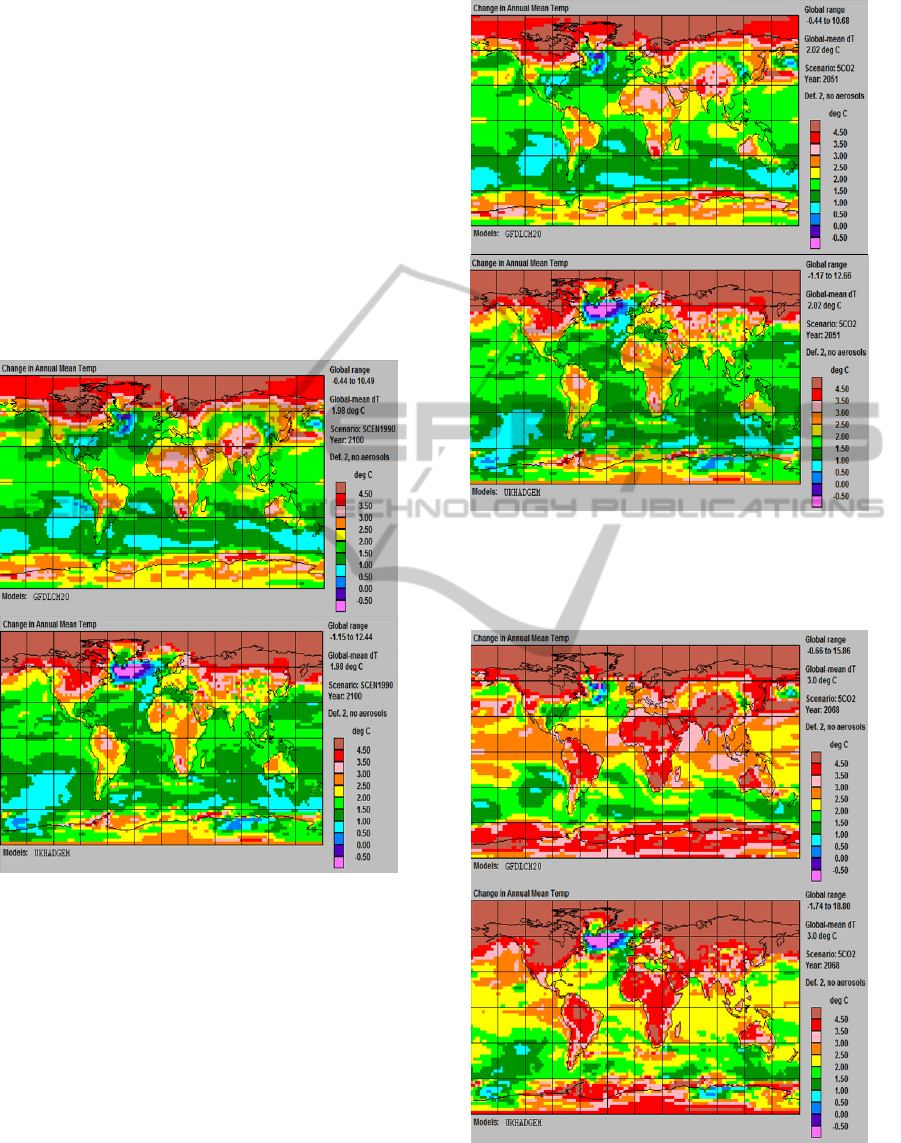
Figure 7: Spatial distribution of T= 1.01 °C according to
GFDL 2.0 (upper panel) and HADGEM1 (lower panel) for
0CO2 emission trajectory (SCEN1990 in map). Maps
were obtained using Magicc/Scengen V. 5.3.
Figure 8: Spatial distribution of T= 1.01 °C according to
GFDL 2.0 (upper panel) and HADGEM1 (lower panel) for
5CO2 emission trajectory. Maps were obtained using
Magicc/Scengen V. 5.3.
NaturalHandlingofUncertaintiesinFuzzyClimateModels
541
Now that we have the temperatures and the
uncertainty intervals we use the Magicc/Scengen to
obtain the maps for the temperatures referred above.
This is done next.
As an example the results for the GCMs:
(Geophysical Fluid Dynamics Laboratory Coupled
Model, version 2.0) GFDL 2.0 and (Hadley Centre
Global Environmental Model version 1) HADGEM1
for 1, 2, 3 and 4 °C are shown (figures 7 to 12).
The maps obtained with Magicc/Scengen for the
HADGEM1 model for an increase of 1.01 °C (and
for T 2 °C) with 5 and 0 CO2, are almost
identical, as expected; the same for the GFDL2.0, i.
e., they are independent from the emission
trajectories.
Figure 9: Spatial distribution of T= 1.98 °C according to
GFDL 2.0 (upper panel) and HADGEM1 (lower panel) for
0CO2 emission trajectory (SCEN1990 in map). Maps
were obtained using Magicc/Scengen V. 5.3.
Once we have temperatures, uncertainty intervals
and two dimensional maps we can go back to the
original question, but put in different terms. When is
the temperature going to be one degree warmer than
today? The answer: as soon as 2021 but there is the
possibility of a larger increase. A picture of the
warming can be imagined between maps of upper
and lower panels shown in Figures 7 or 8. Now if
the temperature is 2 degrees? The answer is that all
the maps shown in the figures would become
possible.
Figure 10: Spatial distribution of T= 2.02 °C according
to GFDL 2.0 (upper panel) and HADGEM1 (lower panel)
for 5CO2 emission trajectory. Maps were obtained using
Magicc/Scengen V. 5.3.
Figure 11: Spatial distribution of T= 3.0 °C according to
GFDL 2.0 (upper panel) and HADGEM1 (lower panel) for
5CO2 emission trajectory. Maps were obtained using
Magicc/Scengen V. 5.3.
SIMULTECH2013-3rdInternationalConferenceonSimulationandModelingMethodologies,Technologiesand
Applications
542
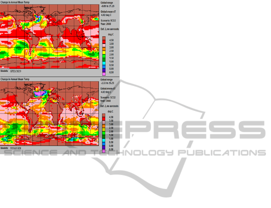
Figure 12: Spatial distribution of T= 4.02 °C according
to GFDL 2.0 (upper panel) and HADGEM1 (lower panel)
for 5CO2 emission trajectory). Maps obtained using
Magicc/Scengen V. 5.3.
4 CONCLUSIONS
Based on the fuzzy model presented by Gay et al.
(2013) and the simple climate model contained in
Magicc/Scengen we show how the global mean
temperature increase is distributed on the globe for
the significant thresholds of 1, 2, 3 and 4 °C. The
linear emission pathways include all the possibilities
mentioned in successive reports of IPCC.
In this work we considered the possibility of
analysing the impacts of temperature increase from
the perspective of the year in which some
temperature is reached. Two sources of uncertainty
are taken into account, the emissions of GHG and
the climate sensitivity.
The larger concentration and sensitivity the
sooner the successive thresholds of temperature will
be reached. If the sensitivity is 6 there is no way of
staying at two degrees unless the concentrations of
CO2 had followed the -2CO2 trajectory: negative
emissions that means very strong subtraction of CO2
from the atmosphere. We think that it is easier to
consider a degree by degree strategy than one based
on dates. For a one degree global increase the
uncertainty extends to more than two degrees, then
for a 1 °C global increase, maps for one and two
degrees are to be considered. For 4 °C and
sensitivity 3, uncertainty can extend to 6.41 °C
We construct maps for 2 GCM´s (as an example)
with the necessary concentration to reach 1, 2, 3 and
4 °C limits to 2100. The maps show the spatial
distribution of the temperature increase over the
globe.
Emissions and sensitivity introduce uncertainties
in the temperature that in turn must be reflected in
the scaled temperature displayed in a map. Other
source of uncertainty considered is the GCM. As
expected, the map for any limit of temperature
depends on the GCM but not on the emission
trajectory. The maps constructed for different
GCM´s illustrate all possibilities for a region of the
globe.
Future work can be done to show how the
GCM´s introduce uncertainty in the estimates of
temperature increase in a regional scale.
ACKNOWLEDGEMENTS
This work was supported by the Programa de
Investigación en Cambio Climático (PINCC,
www.pincc.unam.mx) of the Universidad Nacional
Autónoma de México.
REFERENCES
Gay, C., Sánchez, O., Martínez-López, B., Nébot, Á.,
Estrada, F. 2012. Simple Fuzzy Logic Models to
Estimate the Global Temperature Change due to GHG
Emissions. 2nd International Conference on
Simulation and Modeling Methodologies,
Technologies and Applications (SIMULTECH).
Special Session on Applications of Modeling and
Simulation to Climatic Change and Environmental
Sciences - MSCCEC 2012. July 28-31. Rome, Italy.
Thomson Reuters Conference Proceedings Citation
Index (ISI), INSPEC, DBLP and EI (Elsevier Index)
http:// www.informatik.uni-trier.de/~ley/db/conf/
simultech/simultech2012.html
Gay, C., Sánchez, O., Martínez-López, B., Nébot, Á.,
Estrada, F. 2013. Fuzzy Models: Easier to Understand
and an Easier Way to Handle Uncertainties in Climate
Change Research. In: Simulation and Modeling
Methodologies, Technologies and Applications.
Volume Editor(s): Pina, N., Kacprzyk, J. and Filipe, J.
In the series "Advances in Intelligent and Soft
Computing". Springer- Verlag GmbH Berlin
Heidelberg (in review).
IPCC-WGI, 2007: Climate Change 2007: The Physical
Science Basis. Contribution of Working Group I to the
Fourth Assessment Report of the Intergovernmental
NaturalHandlingofUncertaintiesinFuzzyClimateModels
543

Panel on Climate Change [Solomon, S., D. Qin, M.
Manning, Z. Chen, M. Marquis, K.B. Averyt, M.
Tignor and H.L. Miller (eds.)] Cambridge University
Press, Cambridge, United Kingdom and New York,
NY, USA, 996 pp.
Nakicenovic, N., J. Alcamo, G. Davis, B. de Vries, J.
Fenhann, S. Gaffin, K. Gregory, A. Grübler, T. Y.
Jung, T. Kram, E. L. La Rovere, L. Michaelis, S.
Mori, T. Morita, W. Pepper, H. Pitcher, L. Price, K.
Riahi, A. Roehrl, H.-H. Rogner, A. Sankovski, M.
Schlesinger, P. Shukla, S. Smith, R. Swart, S. van
Rooijen, N. Victor, Z. Dadi, 2000. Special Report on
Emissions Scenarios: A Special Report of Working
Group III of the Intergovernmental Panel on Climate
Change. Cambridge University Press, Cambridge, 599
pp.
Wigley T. M. L., 2008. MAGICC/SCENGEN 5.3: User
Manual (version 2). NCAR, Boulder, CO. 80 pp. (on
line: http://www.cgd.ucar.edu/cas/wigley/magicc/)
Zadeh, L. A. 1965. Fuzzy Sets: Information and Control.
Vol. 8(3) p. 338-353.
SIMULTECH2013-3rdInternationalConferenceonSimulationandModelingMethodologies,Technologiesand
Applications
544
