
Adaptive Deployment of a Mobile Sensors Network to Optimize
the Monitoring of a Phenomenon Governed by Partial Differential
Equations
Alban Vergnaud
1
, Philippe Lucidarme
1
, Laurent Autrique
1
and Laetitia Perez
2
1
LISA, ISTIA, Université d’Angers, 62 avenue Notre Dame du Lac, 49000 Angers, France
2
LTN, UMR 6607, Rue C. Pauc - BP 50609 - 44306 Nantes Cedex 3, France
Keywords: Mobile Sensor Network, Partial Differential Equations, Optimal Control, Experimental Prototype.
Abstract: This project is intended to develop a comprehensive methodology (theory and numerical methods) in order
to achieve an optimal design of experiments in the context of nonlinear ill posed problems related to the
evaluation of parameters in systems described by partial differential equations (PDE). An experimental
prototype will be developed in order to validate the performance of different strategies to identify location
of one (or more) heating source using a set of mobile sensors.
1 STAGE OF THE RESEARCH
This project is intended to develop a comprehensive
methodology (theory and numerical methods) in
order to achieve an optimal design of experiments in
the context of nonlinear ill posed problems related to
the evaluation of parameters in systems described by
partial differential equations (PDE). An
experimental prototype will be developed in order to
validate the performance of different strategies to
identify location of one (or more) heating source
using a set of mobile sensors.
2 OUTLINE OF OBJECTIVES
The protection of the environment and people
requires the use of sensors to monitor the movement
of mobile phenomena to predict and act on their
evolution (ex: polluting cloud, fires, oil slick). These
physical phenomena are often modeled by non-
linear partial differential equations. Development of
a predictive tool for the decision support requires the
assessment of some input parameters.
In these cases, the sensors are generally
expensive and in limited numbers. However, recent
technological advances for communication systems
and miniaturization will result in a cost reduction.
Thus, it becomes possible to develop low-cost
mobile systems and deploy a group of networked
vehicles in a number of environments at risk. Our
aim is to develop and validate optimal strategies to
move a set of sensors for the parametric
identification of PDE systems.
Three major objectives emerge from this
research project:
- Define a set of methods to propose optimal
strategies of mobile sensors movement dealing
with conflicts of trajectories, the environmental
constraints (no-go areas), duplication of
information.
- Design, construction and validation of an
experimental device to validate the deployments
strategies using sensors embedded on mobile
robots.
- Development and implementation of controls
distributed to mobile robots so as to have a set of
autonomous and intelligent vehicles without
centralized control
3 RESEARCH PROBLEM
Disciplinary fields needed for the success of this
project are varied: analysis of dynamical systems,
robotics, and identification in thermal engineering.
The trajectories of mobile sensors will be selected
considering a set of points whose interest will be
quantified online considering sensitivity functions. It
8
Vergnaud A., Lucidarme P., Autrique L. and Perez L. (2013).
Adaptive Deployment of a Mobile Sensors Network to Optimize the Monitoring of a Phenomenon Governed by Partial Differential Equations.
In Doctoral Consortium, pages 8-14
DOI: 10.5220/0004637400080014
Copyright
c
SciTePress

comes to send sensors on the most relevant areas
collecting information on target phenomenon.
Strategies are defined by solving systems of partial
differential equations modeling the dynamics of the
phenomenon being studied. This resolution must be
fast enough given the movement speed of the target
(pollutants...), the time of acquisition of the sensors
and the speed of the robots mobile media sensors.
4 STATE OF THE ART
The determination of models of dynamic systems is
an essential step for the optimization of complex
processes. Such problems typically involve systems
of differential equations and are commonly used in
chemical processes, robotics, electrical engineering,
mechanical engineering, etc. However, the complex
process control frequently requires models more
accurate in which both the spatial dynamic and the
temporal dynamic must be taken into account. Such
systems are often called distributed parameters
systems (DPS) and they are described by PDE (often
non-linear and involving different phenomena).
They are common for example in air quality control
systems, management of groundwater resources,
calibration of models in meteorology, oceanography
or thermal engineering.
One of the fundamental questions in the study of
the DPS is the determination of unknown parameters
of the model from observed data of the real system.
In such an aim, it is usual to develop a mathematical
model and a numerical tool so that the predicted
theoretical responses are closest as possible of those
of the real system collected by appropriate sensors.
A major difficulty is that it is difficult to observe the
variables of interest of the process on the whole
space. The question then arises of the optimal
placement of sensors which allow a reconstruction
as relevant as possible to the state of the process. In
addition, most of the possible locations for the
sensors is rarely specified in the design. Finally,
observations are tainted with inaccuracy due to the
acquisition chain as well as the noisy environment.
All the above-mentioned points make this issue
particularly attractive. The location of sensors is not
necessarily dictated by physical considerations or by
intuition and, therefore, systematic approaches
should be developed to reduce the cost of
instrumentation and increase the efficiency of
estimators.
Although the requirement for systematic
methods has been widely recognized, most of the
techniques available in the literature are based on a
comprehensive search from a set of pre-determined
points. This approach is possible when the number
of measurements is relatively low, but becomes
quickly inadequate to more complex situations.
Adopted optimization criteria are generally based on
the Fisher Information Matrix (FIM) associated to
the unknown considered parameters. The idea is to
express the validity of the estimated parameters
considering the covariance matrix of the evaluations.
To identify optimal sensor placements, it is assumed
that an unbiased estimator is implemented. This
leads to a great simplification since Cramér-Rao
limit of the covariance matrix is the inverse of the
FIM, which can be calculated relatively easily,
although the exact covariance of a given estimator
matrix is difficult to obtain. Fedorov has directed
works based on this approach in the early 1970s.
This methodology has been considerably developed
to extend it to various application fields. An
comprehensive treatment of both theoretical and
numerical aspects of the resulting sensor placement
strategies is presented in (Ucinski, 2005).
To evaluate the parameters, the maximum
likelihood (ML) estimator can be used. Due to the
nonlinear nature inherent in this optimization,
specific numerical techniques should be used. In
addition, when the number of parameters to evaluate
is important, the evaluation problem is ill-posed in
the sense that measurement noise can cause
significant variations in the estimated parameters
and does not ensure the uniqueness. In this context,
known techniques have been developed such
regularization methods (Tikhonov-Phillips). While
ill posed character of this type of problem is
common in many industrial processes, systematic
design of experimental conditions ensuring an
optimal observation has received very little attention
so far. Generally, existing approaches adopt an ideal
perspective ignoring the ill-posed nature. Then, they
could provide reasonable designs in some situations.
However, they lead in general to non-optimal
experimental solutions that can in some cases prove
to be false qualitatively. This gap between theory
and practice for the optimum
placement of sensors is
the main motivation of this research project
Different works allowed to propose paths of
sensors (ensuring a continuous spatial scan for
example). In the latter case even if the complexity of
the resulting optimization problem is larger, it may
be interesting that sensors are able to track the points
that provide the most relevant information at any
given time. Therefore, by reconfiguring in real time
a sensor system (moving) we can expect to obtain an
optimality criterion better than that of the stationary
AdaptiveDeploymentofaMobileSensorsNetworktoOptimizetheMonitoringofaPhenomenonGovernedbyPartial
DifferentialEquations
9

case.
5 METHODOLOGY
The thermal context that allows studying PDE's
parabolic types possibly non-linear has been selected
for the study of this research project. Numerous
studies have been performed in one dimensional
geometry (Silva Neto and Özisik, 1994),(Yi and
Murio, 2002),(Hasanov, 2012) as well as in two
dimensional domain (Khachfe and Jarny, 2000),
(Ling et al., 2006) and (Yang, 2006).
5.1 Direct Problem Formulation
The studied domain is a thin metallic square plate.
Let us consider that thickness
e
is quite small and
that temperature gradients versus the thickness are
neglectable. The studied geometry is denoted by
2
,0,
x
yL
and time variable is denoted by
0,
f
tT T
,
f
T is the final time. Several heat
sources
j
S
1, ,
s
jN
move on the surface of
the plate. For each source, the density flux
j
t
is
assumed to be uniform on a disk
,
jj
D
Itr
with
(centre
,
jjj
I
txtyt
and radius of a few
centimeters. The total heating flux can be expressed
by:
1
if ,
Φ ,;
0otherwise
s
N
j
j
j
txyD
xyt
(1)
To describe the heat flux in continuous and
differentiable manner, spatial regularization is
considered:
Φ .atan.
2
j
j
j
t
r
(2)
where
22
,,
jjj
x
yt x x t y y t
.
The regularization parameter
was chosen so as to
accurately describe the discontinuity at each heating
disk boundary. The time interval is divided into
segments as follows:
1
0
0, ,
t
N
fii
i
ttt
, with time
i
ti
and step time
1
f
t
t
N
. Discretization of the
heating flux is also proposed according to
continuous linear piecewise function:
1
1
1if ,
1if ,
0otherwise
ii
iii
t
ittt
t
tittt
Trajectories and heat fluxes are thus parameterized
as follows:
1
1
1
t
t
t
N
tr
j
j
jii
i
N
tr
j
jiij
i
N
tr
j
jiij
i
x
txtxt
y
tytyt
ttt
The spatio-temporal distribution of temperature
,;
x
yt
within the domain is solution of the
following system of partial derivatives equations:
,; 0,
f
x
yt T
(3)
0
.2 .
.
.
h
c
te
,xy
0
,;0xy
,; 0,
f
x
yt T
.
0
n
where
-3 -1
J.m .Kc
is the volumetric heat
capacity,
-1 -1
W.m .K
the thermal conductivity,
-2 -1
W.m .Kh
the convective exchange coefficient,
0
K
the initial temperature equal to the ambient
one. When all parameters are known, temperature
evolutions in the plate are predicted considering the
numerical resolution of the previous direct problem
using the Comsol ® interfaced Matlab © software.
5.2 Inverse Problem
To identify the successive positions of the centers
1, ,
,
s
jj
j
N
Ixy
as well as the heating flux
1, ,
s
j
j
N
of each of j sources from the
ICINCO2013-DoctoralConsortium
10

observations provided by
c
N mobile sensors
p
C ,
an inverse problem is solved by minimizing the
quadratic criterion between calculated
,; ,
p
CtI
and measured temperatures:
ˆ
p
t
2
0
1
ˆ
,, ,;,
2
f
T
pp
p
J
ICtItdt
4
Considering that initial positions of the sources are
known:
0, 0
jj
xy
, a method of iterative
regularization based on Conjugate gradient
algorithm is implemented (Perez et al., 2008). The
resolution algorithm requires iterative resolution of
three well problems in the Hadamard’s sense
(Alifanov et al., 1995) and (Tarantola, 2005):
-
The direct problem to calculate the test and judge
the quality of the estimate.
-
The adjoint problem to calculate the gradient of the
test and thus to define the next direction of
descent.
-
The sensitivity problem to calculate the depth of
descent (in the direction of descent).
The crucial steps that are the resolution of the
sensitivity problem and the computation of the
gradient functional by the adjoint problem resolution
are detailed hereafter (See (Huang and Wang, 1999),
(Huang and Chen, 2000), (Autrique et al., 2005) and
(Beddiaf, 2012) for examples related to parametric
identification.
5.2.1 Sensitivity Problem
The temperature variation caused by variation in
centres disks
1, ,
,
s
jj
j
N
Ixy
and the heat
fluxes
1, ,
s
j
j
N
of each of the j sources is
noted
,;δθ xyt
and is solution of the sensitivity
problem:
,; 0,
f
x
yt T
(5)
..2.
.
h
c
te
,xy
,;0 0xy
,; 0,
f
x
yt T
.
0
n
with:
2
2
Φ ,;
1
atan .
2
1
1.
1
1.
tr
jj
j
tr tr tr
jjj
j
j
tr tr tr
jjj
j
j
xyt
tr
txtxtx
r
tytyty
r
where:
22
,,
tr tr
jjj
xyt x x t y y t
.
Thus, at iteration
1k
, the depth of descent
1k
in
the direction of descent
1k
d
can be expressed by :
(Beddiaf, 2012).
1
1
1
0
2
0
,; ,
,; ,
f
k
f
k
T
kkk
pp
d
p
k
t
kk
p
d
p
Et CtI dt
CtI dt
(6)
where
ˆ
,; ,
kkk
pp p
Et CtI t
.
The sensitivity problem
5
has to be numerically
solved at each iteration
1k
in the descent direction
1k
d
in order to calculate the descent depth
1k
according to relation
6
.
5.2.2 Adjoint Problem
A Lagrangian formulation
,,I
for the
quadratic function minimization based on an adjoint
function
,;
x
yt
is introduced in order to
determine the functional gradient for each iteration
of the minimization algorithm (Perez et al., 2008;
Beddiaf et al., 2012; Rouquette et al., 2007):
AdaptiveDeploymentofaMobileSensorsNetworktoOptimizetheMonitoringofaPhenomenonGovernedbyPartial
DifferentialEquations
11
0
0
,,, ,,
2
f
t
IJI
h
cdxdydt
te
Let us introduce
,
p
C
x
y
is the Dirac distribution
at mobile sensors
p
C , then :
2
0
0
0
,,,
1
ˆ
.; , ,
2
2
f
p
f
t
pC
p
t
I
I
txydxdydt
h
cdxdydt
te
Thus,
,,,II
I
If the temperature
,,
x
yt
is the solution of the
direct problem
3
then
,,, ,,IJI
and
,,, ,,IJI
. If the Lagrange
multiplier
,,
x
yt
is fixed then
0
.
Moreover
,,
x
yt
is fixed such that
0
. Considering boundary conditions
of the sensitivity problem
,,
x
yt
has to be
solution of the adjoint problem:
,; 0,
f
x
yt T
(7)
.
2
.. .
h
cE
te
,xy
,; 0
f
xyT
,; 0,
f
x
yt T
.
0
n
with
ˆ
,, ,; ,
p
pC
p
E xyt xyt t xy
,
thus:
0
.
f
T
I dxdydt
e
I
.
As
,,, ,,IJI
then the gradient of
the criterion can be obtained from the resolution of
7
and the next descent direction can be calculated.
Both adjoint and sensitivity problems can be solved
at each iteration with the same numerical scheme as
for the direct problem.
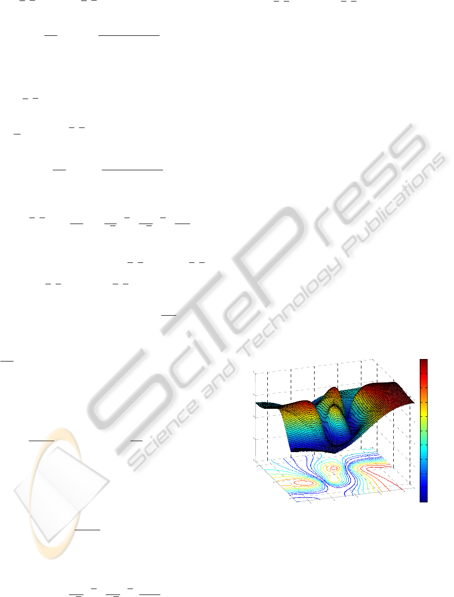
5.3 Observation Strategies
The previous paragraph has allowed to define the
methodology of identification based on solving
iteratively three well-posed problems. The success
of this research project partially rely on the
observations strategy and more specifically on the
movement of mobile sensors. These displacements
are planned from the two following approaches:
-
Implementation of a sliding horizon for the
identification based on the iterative regularization
of the Conjugate gradient method, in order to
update the trajectories of sensors based on
estimates of the unknown parameters,
-
Analysis of the evolution of sensitivity
distributions obtained by iterative resolution of the
sensitivity problem in order to define the new areas
of interest for the process observations.
An example of such distributions is presented on
figure 1: depending on the number of sensors and
their previous positions, strategies of displacement
can be proposed.
-0.02
0
0.02
-0.02
-0.01
0
0.01
0.02
-1
-0.5
0
0.5
1
y
in m
x
in m
0.1
0.2
0.3
0.4
0.5
0.6
0.7
0.8
0.9
1
Figure 1: Example of spatial distribution of sensitivity
(normalized).
5.4 Experimental Prototype
To assess the different strategies of positioning
sensors and before considering the application on a
large scale (ex: detection of pollutants), an
ICINCO2013-DoctoralConsortium
12
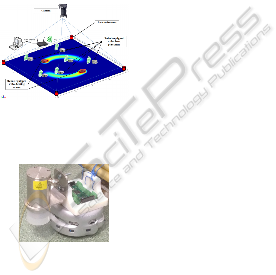
experimental device is currently under development.
In such a way, several heating sources embedded on
mobile robots (Khepera III) evolve on a plane
surface and provide the heating of a thin plane
material (figure 2) on a surface of approximately 4
m². The time dependant heat flux of these heat
sources can be controlled in order to reach
temperatures for which the thermal properties of the
material are thermo-dependent (introducing non-
linearity).
Figure 2: Representation of the experimental prototype.
On this same surface several mobile robots will be
equipped with pyrometers laser (figure 3) to measure
the temperature of the plate on a small area (a few
mm2).Their locations and the measured temperature
will be transmitted to a central computer via a
wireless (WIFI) technology.
Figure 3: Khepera robot equipped with a Laser pyrometer.
In order to accurately measure the robots location on
the material surface, a camera will be placed above
the plate and then by image processing (Martinez-
Gomez and Weitzenfel, 2004; Zickler et al., 2009;
Wang et al., 2001) the positions of different robots
will be returned to the computer that will
synchronize the received measures of robots with
their positions. This positioning by tag system
comes in addition to the position data sent from the
robots in order to take into account odometry errors
that may be encountered while displacements.
6 EXPECTED OUTCOME
In this communication, the DARC-EDP project is
presented as a whole. It deals with the deployment
of mobile sensors to identify moving heating sources
in the context of thermal engineering. Several points
have been briefly addressed:
-
modeling heat transfers and direct problem
formulation
-
inverse problem formulation,
-
minimization by a descent method : iterative
regularization based on conjugate gradient method
(sensitivity problem and adjoint problem),
-
observations strategies,
-
design of the experimental prototype.
The prospects for these works consist of the
confrontation of experimental campaigns with the
previous numerical studies.
REFERENCES
Alifanov O. M., Artyukhin E.A., Rumyantsev S. V., 1995
“Extreme Methods for solving Ill Posed Problems with
Applications to Inverse Heat Transfer Problems”,
(1995), Begell House, New York.
Autrique L., Ramdani N., Rodier S., 2005 “Mobile source
estimation with an iterative regularization method”,
5th International Conference on Inverse Problems in
Engineering: Theory and Practice, Cambridge, UK,
11-15 July, (2005), 1, pp A08
Beddiaf S., Autrique L., Perez L., Jolly J. C., 2012
“Heating sources localization based on inverse heat
conduction problem resolution”, Sysid 2012, 16th
IFAC Symposium on System Identification, Bruxelles.
Beddiaf S., Autrique L., Perez L., Jolly J. C., 2012 “Time-
dependent heat flux identification: Application to a
three-dimensional inverse heat conduction problem”,
4th International Conference on Modelling,
Identification and Control (IEEE Conference
Publications), June 24-26, 2012, Wuhan- China, pp.
1242 – 1248.
Hasanov A., 2012 “Identification of spacewise and time
dependent source terms in 1D heat conduction
equation from temperature measurement at a final
time”, International Journal of Heat and Mass
Transfer, 55, (2012), pp. 2069 – 2080.
Huang C. H., Wang S. P., 1999 “A three-dimensional
inverse heat conduction problem in estimating surface
AdaptiveDeploymentofaMobileSensorsNetworktoOptimizetheMonitoringofaPhenomenonGovernedbyPartial
DifferentialEquations
13

heat flux by conjugate gradient method”, International
Journal of Heat and Mass Transfer, 42, (1999), pp.
3387 – 3403.
Huang C. H., Chen W. C., 2000 “A three-dimensional
inverse forced convection problem in estimating
surface heat flux by conjugate gradient method”,
International Journal of Heat and Mass Transfer, 43,
(2000), pp. 317 – 3181.
Khachfe R. A, Jarny Y., 2000 “Numerical solution of 2-D
nonlinear inverse heat conduction problems using
finite-element techniques”. Numerical Heat Transfer -
Part B, vol 37- 1 (2000) 45-67
Ling L., Yamamoto M., Hon Y. C, Takeuchi T., 2006
“Identification of source locations in two-dimensional
heat equations”, Inverse Problems, 22, (2006), pp.
1289 – 1305.
Martinez-Gomez L.A., Weitzenfeld A., 2004 “Real Time
Vision System for a Small Size League Team”,
Proceedings of the 1st IEEE Latin American Robotics
Symposium – LARS, Mexico city, October 28 – 29,
2004 , Mexico.
Perez L., Autrique L., Gillet M., 2008 “Implementation of
a conjugate gradient algorithm for thermal diffusivity
identification in a moving boundaries system”, Journal
of physics, Conference series, Vol. 135,
doi:10.1088/1742-6596/135/1/012082.
Rouquette S., Autrique L., Chaussavoine C., Thomas L.,
2007 “Identification of influence factors in a thermal
model a plasma assisted chemical vapour deposition
process”, Inverse Problems in Science and
Engineering, Vol. 15, n° 5, pp. 489-515.
Silva Neto A. J, Özisik M. N., 1994 “The estimation of
space and time dependent strength of a volumetric
heat source in a one-dimensional plate”, International
Journal of Heat and Mass Transfer, 37, (1994), pp. 909
– 915.
Tarantola A., 2005 “Inverse Problem Theory and Methods
for Model Parameter Estimation”, (2005), Society for
Industrial and Applied Mathematics (SIAM)
publication.
Ucinski D, 2005 “Optimal Measurement Methods for
Distributed Parameter System Identification”, CRC
Press, 2005.
Wang C., Wang H., Soh W. Y. C., Wang H., 2001 “A Real
Time Vision System for Robotic Soccer”, 4th Asian
Conference on Robotics and its application,
Singapour.
Yang C. Y., 2006 “The determination of two moving heat
sources in two-dimensional inverse heat problem”,
Applied Mathematical Modelling, 30, (2006), pp. 278
– 292.
Yi Z. H, Murio D. A., 2002 “Source term identification in
1D IHCP”, Computers and Mathematics with
Applications, 47, (2002), pp. 1921 – 1933.
Zickler S., Laue T., Birbach O., Wongphati M., Veloso
M., 2009 “SSL-Vision: The Shared Vision System for
the RoboCup Small Size League”, RoboCup 2009:
Robot Soccer World Cup XIII, 425-436, Springer.
ICINCO2013-DoctoralConsortium
14
