
A Computational Model of Grid Cells based on
Dendritic Self-organized Learning
Jochen Kerdels and Gabriele Peters
Chair of Human-Computer Interaction, University of Hagen, Universit
¨
atsstrasse 1 , D-58097 Hagen, Germany
Keywords:
Grid Cells, Model of Grid Formation, Self Organization, Population Coding.
Abstract:
In this paper we present a new computational model for grid cells. These cells are neurons in the entorhinal
cortex of the hippocampal region that encode allocentric spatial information. They possess a peculiar, trian-
gular firing pattern that spans the entire environment with a virtual lattice. We show that such a firing pattern
can emerge from a dendritic, self-organized learning process. A key aspect of the proposed model is the hy-
pothesis that the dendritic tree of a grid cell can behave like a sparse self organizing map that tries to cover its
input space as best as possible. We argue, that the encoding scheme used by grid cells is possibly not limited
to the description of spatial information and may represent a general principle on how complex information is
encoded in higher level brain areas like the hippocampal region.
1 INTRODUCTION
In recent years several types of neurons were discov-
ered in the hippocampal region, notably in the en-
torhinal cortex, that encode allocentric spatial infor-
mation. Among those newly discovered types of neu-
rons are so-called grid cells. These neurons exhibit
a peculiar kind of firing pattern. Every grid cell cov-
ers the entire environment of the animal with a vir-
tual, triangular lattice and whenever the animal passes
through a vertex of this lattice, the grid cell fires. A
common hypothesis suggests that groups of grid cells
with lattices of different scale and orientation collec-
tively encode a single, absolute position of the animal
(McNaughton et al., 2006; Fiete et al., 2008; Moser
et al., 2008).
In this paper we present a new computational
model for grid cells that illustrates how the triangu-
lar firing pattern of these cells can emerge from a
dendritic, self-organized learning process. A key as-
pect of this model is the hypothesis that the dendritic
tree of a grid cell behaves like a sparse self organiz-
ing map that tries to cover its input space as best as
possible. This conceptual shift from common self-
organized maps on a neuronal network level to in-
dividual self-organized maps per neuron holds some
interesting new perspectives on how complex, high
level information may be represented within popula-
tions of neurons. We argue, that the encoding scheme
used by grid cells is possibly not limited to the de-
scription of spatial information and may represent a
general principle on how complex information is en-
coded in higher level brain areas like the hippocampal
region.
The paper is organized as follows: Sections 2
and 3 will briefly summarize key elements and prop-
erties of the spatial representation in the hippocampal
region in general and of grid cells in particular. In sec-
tion 4 an overview of existing computational models
for grid cells is given. Subsequently we introduce our
own computational model in section 5 and provide ex-
perimental results in section 6 that further illustrate
the properties of the proposed model. The paper ends
with a more general discussion and an outlook on fur-
ther research directions in sections 7 and 8.
2 SPATIAL REPRESENTATION IN
THE HIPPOCAMPAL REGION
The hippocampal region
1
of the mammalian brain
contains several types of neurons that encode allo-
centric spatial information. In 1971 O’Keefe and
Dostrovsky made the discovery of place cells in rats
(O’Keefe and Dostrovsky, 1971; O’Keefe, 1976).
These cells, located in the CA1 and CA3 regions of
the hippocampus, fire when the animal passes through
1
A good overview of the hippocampal region is given in
(Witter et al., 2000; van Strien et al., 2009).
420
Kerdels J. and Peters G..
A Computational Model of Grid Cells based on Dendritic Self-organized Learning.
DOI: 10.5220/0004658804200429
In Proceedings of the 5th International Joint Conference on Computational Intelligence (NCTA-2013), pages 420-429
ISBN: 978-989-8565-77-8
Copyright
c
2013 SCITEPRESS (Science and Technology Publications, Lda.)

specific locations in its environment. The location
where a particular place cell fires is called the cell’s
place field.
In 1990 Taube et al. presented their finding of
head-direction cells in rats (Taube et al., 1990). As
their name suggests head-direction cells fire when
the animal is looking in a certain, absolute direction.
Head-direction cells were found in several brain re-
gions including the postsubiculum, anterodorsal tha-
lamus, lateral mammillary nuclei, retrosplenial cor-
tex, lateral dorsal thalamus, striatum, and entorhinal
cortex (Taube, 2009). The absolute firing direction
of these cells is controlled by different, external cues
such as visual landmarks. Additionally, internal self-
motion information like angular head velocity is in-
tegrated to maintain head direction information when
external cues are less available, e.g., when the animal
moves in the dark.
Another cell type similar to place cells are grid
cells (Fyhn et al., 2004; Hafting et al., 2005). They
are located in the medial entorhinal cortex. In con-
trast to place cells grid cells have not one but several
firing fields which are arranged in a periodic triangu-
lar grid that spans the entire environment of the ani-
mal (Fig. 1). It is commonly assumed that grid cells
participate in a path integration computation that de-
termines the absolute position of the animal in its en-
vironment using speed and direction signals as input.
A more detailed description of grid cell properties and
a summary of current theoretical models of grid cell
formation are given in section 3 and section 4, respec-
tively.
In addition to grid cells further investigation of the
entorhinal cortex revealed the existence of grid cells
colocalized with head-direction cells and conjunctive
grid × head-direction cells (Sargolini et al., 2006) as
well as border cells (Solstad et al., 2008). The lat-
ter being a cell type that fires whenever the animal
is close to a physical border in its environment, e.g., a
wall. Conjunctive grid × head-direction cells are cells
with grid-cell-like firing fields that only fire at those
field locations when the animal is facing in a certain
direction.
3 GRID CELLS
The first detailed account of grid cells in the medial
entorhinal cortex (MEC) of rats was given by Hafting
et al. in (Hafting et al., 2005). Grid cells encode al-
locentric spatial information as they exhibit multiple
discrete firing fields, i.e., they only fire when the an-
imal moves through certain positions of its environ-
ment. The firing fields of a single grid cell are ar-
ranged in a very peculiar, triangular grid that spans
the entire environment. Figure 1 depicts the firing
pattern of such a grid cell while a rat is moving in
a square enclosure. The trajectory of the rat is rep-
resented by the black lines, firing of the place cell at
a given location is indicated by a red dot. The right
side of the figure shows the spatial autocorrelation of
the grid cell’s firing rate map (not shown) with blue
colors representing low values and red colors repre-
senting high values.
Figure 1: Left: the black line represents the running path of
a rat. Spikes fired by a single grid cell at a certain position
are marked with a red dot. Right: color coded spatial auto-
correlation (blue: low values, red: high values) of the grid
cell’s rate map (not shown) verifying the periodic triangu-
lar firing pattern of the grid cell. Images by Torkel Hafting
under CC BY-SA 3.0 licence.
Hafting et al. define four measures to describe the
spatial properties of grid cells: spacing, orientation,
field size, and phase. The spacing of a grid cell is
given by the median of the distances between the cen-
tral peak of the autocorrelogram and its surrounding
six peaks. The orientation of a grid cell is defined
as the angle between a given reference line (0 de-
grees) going through the central peak of the autocor-
relogram and a vector from the central peak to the
surrounding vertex which is nearest to the reference
line in counterclockwise direction. The field size, i.e.,
the size of the individual fields of a grid cell, is es-
timated by the area covered by the central peak of
the autocorrelogram using a fixed threshold as min-
imum value. The phase of a grid cell refers to the lo-
cation of its grid vertices. The notion of a phase stems
from the fact that co-localized grid cells exhibit sim-
ilar spacing, orientation, and field size (see below),
but have different locations for their firing fields. For
two co-localized grid cells their relative phase shift
is defined as the distance between the origin and the
nearest peak in the cross-correlogram of the cells’ rate
maps. The average phase shift between neighboring
grid cells is evenly distributed and appears to be not
linked to the cell’s relative positions.
A recent study by Stensola et al. analysed 968 grid
cells in 15 rats covering up to 50% of the dorsoventral
AComputationalModelofGridCellsbasedonDendriticSelf-organizedLearning
421

axis of the MEC (Stensola et al., 2012). Their findings
show that the spacing of grid cells increases along
the entorhinal dorsoventral axis in a discrete fash-
ion. They indentified four
2
clusters of grid cells or
grid modules with distinct grid spacings of 39.1, 47.9,
65.1, and 96.6 centimeter on average. Given the area
covered by the measurements Stensola et al. estimate
that the number of grid modules within MEC lies in
the upper singe-digit range. Similar to the grid spac-
ing, the identified grid modules also showed discrete
grid orientations, i.e., grid cell orientations within a
module were more similar than grid cell orientations
across modules.
Although the orientation of grid cells is similar
within a grid module, the orientation itself is not fixed.
It is influenced by external cues, e.g., if a promi-
nent visual cue in a circular environment is rotated
by 90 degrees the orientation of the grid cells will ro-
tate similarly (Hafting et al., 2005). A related phe-
nomenon is reported by (Fyhn et al., 2007; Monaco
and Abbott, 2011). If the environment of the animal
changes significantly, the grid cells exhibit a realign-
ment that is expressed by a change of phase and ori-
entation. Experiments with rats in hairpin mazes in-
dicate, that the realignment is not random but instead
corresponds coherently to geometric properties of the
environment (Derdikman et al., 2009).
In addition to a change of phase and orientation
upon entering a novel environment, Barry et al. de-
scribe a temporary increase in spacing and field size
as well as a reduction in grid regularity (Barry et al.,
2012). Grid scale gradually returned to the values ob-
served in familiar environments after 5 days with 60
minutes of exposure to the novel environment per day.
Wills et al. and Langston et al. investigated the de-
velopment of head-direction cells, grid cells and place
cells in young rats (Langston et al., 2010; Wills et al.,
2010). They found that grid cells and place cells are
present in a coarse and rudimentary form when young
rat pups leave their nest for the first time
3
and start ex-
ploring their environment. In contrast, head direction
cells are already in a mature state at this point of de-
velopment. Grid cells and place cells stabilize their
spatial representations during the first two weeks of
exploration and exhibit adultlike properties when the
rat reaches about 4 weeks of age.
2
The grid spacing of a fith cluster was too large to con-
firm periodicity.
3
typically at 15 to 16 days after birth
4 EXISTING COMPUTATIONAL
MODELS OF GRID CELLS
In recent years a number of computational models
were proposed that offer several different mechanisms
for the formation of grid-like firing fields and other
properties of grid cells. An extended overview of
these models is given in (Giocomo et al., 2011).
The existing models of grid cells can be divided
into three groups: oscillatory-interference models,
attractor-network models, and models based on self-
organization.
In oscillatory-interference models it is assumed
that each grid cell exhibits a somatic and several den-
dritic membrane-potential oscillations (Burgess et al.,
2007; Zilli and Hasselmo, 2010). The frequency
of the somatic oscillator is thought to correspond
approximately to the so-called theta rythm which
is a widespread periodic signal that can be EEG-
captured throughout the hippocampal region of nu-
merous mammal species including the rat. The fre-
quency of the dendritic oscillators is modulated by
running speed and direction whereas the influence of
the latter is relative to a preferred direction specific to
the particular dendritic oscillator. If these preferred
directions are seperated by a multiple of 60 degrees
a triangular, grid-like firing pattern is formed. An in-
dication against oscillatory-interference models was
given by (Yartsev et al., 2011) who report of grid cells
in the entorhinal cortex of bats in the absence of theta
oscillations.
In attractor-network models the formation of a
grid-like firing pattern emerges from the activity of a
local, two-dimensional, continuous attractor network
(Fuhs and Touretzky, 2006; McNaughton et al., 2006;
Navratilova et al., 2012). In such a network a sta-
ble, local “bump” of activity forms due to a two-
dimensional, Mexican hat connectivity of individual
neurons. This bump of activity can then be “moved”
by the activity of several hidden layers of neurons
which are connected in such a way, that each hid-
den layer moves the bump in a particular, preferred
direction. The hidden layers are “selected” by head-
direction cells corresponding to the preferred direc-
tion of the particular layer and the layer activity is
modulated by the current running speed of the animal.
In that way the two-dimensional continous attractor
represents the position of the animal by integrating
direction and speed signals. In order to generate a pe-
riodic, hexagonal firing pattern, the two-dimensional
attractor network has to have the topology of a torus
that is twisted along its major radius.
Models based on self-organization are less
common than oscillatory-interference and attractor-
IJCCI2013-InternationalJointConferenceonComputationalIntelligence
422
network models. Kropff and Treves (Kropff and
Treves, 2008) describe a model that utilizes a set of
neurons that receives the signal of place cells as in-
put. The dynamics of the set of neurons is controlled
by two components. First, the neurons exhibit a form
of neuronal fatigue that modulates the total synaptic
activation of the neuron. Second, the transfer function
of each neuron is controlled by two global, continu-
ally updated parameters that control the overall mean
activity and sparseness. Learning of synaptic weights
is performed via a hebbian learning rule. The result-
ing neurons show a grid-like firing pattern with sim-
ilar spacing. However, the orientations exhibited by
individual neurons are random contrary to experimen-
tal findings.
Mhatre et al. present a different approach using a
form of self-organized learning (Mhatre et al., 2012).
They postulate a type of cell called stripe cell that
possesses a preferred direction and fires periodically
when an animal moves a fixed distance along that
direction. Coactivation of two stripe cells with dif-
ferent preferred directions occurs, when the periodic
patterns of these cells projected onto each other coin-
cide. Geometrically this coactivation is most frequent
when the preferred directions of the two stripe cells
are seperated by 60 degrees. Mhatre et al. use a self
organizing map to learn this geometric relation among
the set of stripe cells. As a result, the units of the self
organizing map exhibit a grid-like firing pattern.
5 MODEL DESCRIPTION
Most of the existing grid cell models described in the
previous section can explain the experimental find-
ings quite well and provide testable predictions that
can guide further experimental investigation. How-
ever, existing models are also characterized by re-
lying on extensive assumptions about very specific
cell and/or network properties, e.g., the existence of
stripe cells in the model of Mhatre et al., the twisted,
toroidal topology of the two-dimensional attractor-
network models, or the preferred directions in the
oscillatory-interference models.
We propose that the observed properties of grid
cells can be explained with fewer and less specific
assumptions about cell and network properties. In
our model, the characteristic properties of grid cells
are the result of three interacting processes. First, an
input process integrates signals from head-direction
cells and speed cells and generates two periodic, one-
dimensional position signals. Second, the position
signals are learned on a local level independently by
each grid cell with a form of self-organized learning,
and third, a second self-organized learning process on
a network level influences and adjusts the individual
learning processes on the local level.
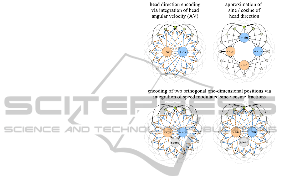
Figure 2: Model for head direction encoding and orthog-
onal, one-dimensional position encoding based on a one-
dimensional continuous attractor network.
Input Level. Like most existing grid cell models
the proposed model uses the current head-direction
and running speed of the animal as input signals.
These signals are then integrated to generate a sig-
nal that represents the current position. We suggest,
that this integration can be achieved by two one-
dimensional, continuous attractor networks. One-
dimensional attrator networks are commonly used to
explain how the activity of head-direction cells can
result from neural integration of angular velocity sig-
nals derived from the vestibular system, e.g., see (Mc-
Naughton et al., 2006). Figure 2 (top-left) depicts
such a model. The outer ring of units represents head-
direction cells. They have excitatory connections to
neighbouring cells that decline in strength with dis-
tance (outer black and grey lines). In addition the set
of head-direction cells is subject to global feedback
inhibition to constrain the overall neural activity. Typ-
ically, such a network forms a single “bump” of ac-
tivity at one location (green colors). This bump can
be moved by a set of hidden units (blue and yellow
ochre) that are asymmetrically connected to the outer
units. The hidden units receive excitatory inputs from
AComputationalModelofGridCellsbasedonDendriticSelf-organizedLearning
423

the outer units and from an input unit, e.g., an angu-
lar velocity (+/- AV) signal. The firing threshold of
the hidden units is assumed to be on a level that re-
quires inputs from both the outer units as well as the
input unit in order to fire. Thus, only the hidden units
“below” the current bump of activity will be active
when an angular velocity signal arrives. This activity
will then move the bump in the direction defined by
the asymmetric connections of the particular hidden
units. As a result, the network can keep track of the
current head direction represented by the outer units.
In order to transform this head-direction signal
into two orthogonal one-dimensional position signals
the sine and cosine fractions of the particular head di-
rections have to be approximated. This approximation
can be achieved by utilizing a well-known electro-
tonic property of neurons. The more distant from the
soma an axonal input to a dendritic tree is, the weaker
is its total effect on the neuron’s activity (Squire et al.,
2008). Figure 2 (top-right) illustrates, how this prop-
erty can be used to approximate the sine and cosine
fractions of the current head direction. The head-
direction cells (outer units) connect to four neurons
that represent the positive and negative parts of a sine
and cosine wave. The connection lengths indicate the
distance to the soma and the corresponding attenua-
tion of the input signals.
Using the sine and cosine fractions and modulat-
ing them with the current running speed of the animal,
the same mechanism described for the integration of
angular velocity signals can be used to generate two
orthogonal, one-dimensional position signals result-
ing effectively in a set of periodic cartesian coordi-
nates of the animal’s position, see figure 2 (bottom).
The cycle period of each coordinate is determined by
the strength of the modulation through the speed sig-
nal.
Local Level. The periodic position signal described
in the previous section is the input to the grid cells
of the proposed model. Considering the increasing
evidence in recent years about the computational ca-
pabilities of dendritic trees (Sjstrm et al., 2008) we
argue that a single neuron – in this case a grid cell –
can learn to represent different inputs within separate
sections of its dendritic tree. A possible mechanism
that could facilitate such a local, dendritic represen-
tation are, e.g., dendritic spikes. As a computational
model of such a dendritic learning process we adopted
the growing neural gas (GNG) described in (Fritzke,
1995). In this context the individual units of the GNG
are thought to be local sections of the dendritic tree of
a grid cell. The adapted GNG approach can be sum-
marized as follows:
The dendritic tree D of a grid cell is described as
a set of dendritic subsections d ∈ D that each have a
reference vector w
d
∈ R
n
and an accumulated error
e
d
∈ R. The reference vector has the dimension n of
the grid cell’s input – in this case the concatenation of
the two one-dimensional position vectors. The struc-
ture of the dendritic tree is implicitly described by a
set of edges c ∈ C that describe the neighbourhood re-
lation that develops between dendritic subsections. In
addition each edge c has an age t
c
∈ N which is ini-
tialized with 0. In the beginning a grid cell has only
two dendritic subsections connected by a single edge.
The reference vectors of these dendritic subsections
are initialized with random values. Each input x to a
grid cell is then processed in the following way:
Find the two dendritic subsection s
1
and s
2
that have
the smallest distance to the input x:
s
1
:= argmin
d
i
∈D
kw
d
i
− xk
s
2
:= argmin
d
j
∈D\
{
s
1
}
kw
d
j
− xk
If there is no edge between s
1
and s
2
add one:
C := C ∪
{
(s
1
,s
2
)
}
Reset the age of the edge between s
1
and s
2
to 0:
t
(s
1
,s
2
)
= 0
Increase the accumulated error of s
1
with the
quadratic distance between the reference vector of s
1
and the input x:
e
s
1
+= kw
s
1
− xk
2
Adapt the reference vectors of s
1
and all dendritic sub-
sections that are connected via an edge with s
1
:
w
s
1
+= ε (x − w
s
1
)
w
d
+= µ · ε (x − w
d
), d ∈
{
a|(s
1
,a) ∈ C,a ∈ D
}
Increase the age of all edges that were “used”:
t
(s
1
,d)
+= 1, d ∈
{
a|(s
1
,a) ∈ C,a ∈ D
}
If the age of an edge if above a given threshold t
max
the
edge is deleted. If this results in a dendritic subsection
that is isolated, the dendritic subsection is removed
too.
Has the number of inputs reached a multiple of a
given parameter λ and is the current number of den-
dritic subsections smaller than a desired maximum
number of dendritic subsections d
max
then a new den-
dritic subsection p will be added to the grid cell.
For this purpose the dendritic subsection q
1
with the
biggest accumulated error is selected as well as the
IJCCI2013-InternationalJointConferenceonComputationalIntelligence
424

dendritic subsection q
2
with the biggest accumulated
error that is connected to q
1
:
q
1
:= argmax
d
i
∈D
e
d
i
q
2
:= argmax
d
j
∈
{
a|(q
1
,a)∈C,a∈D
}
e
d
j
The reference vector w
p
of the new dendritic subsec-
tion p is interpolated between the reference vectors of
q
1
and q
2
:
w
p
:= (w
q
1
+ w
q
2
)/2
The accumulated errors of q
1
and q
2
are reduced and
the accumulated error e
p
of the new dendritic subsec-
tion is interpolated between the reduced errors of q
1
and q
2
:
e
q
1
−= αe
q
1
e
q
2
−= αe
q
1
e
p
:= (e
q
1
+ e
q
2
)/2
The edge between q
1
and q
2
is removed and new
edges between q
1
and p as well as q
2
and p are in-
serted:
C := C \
{
(q
1
,q
2
)
}
C := C ∪
{
(q
1
, p),(q
2
, p)
}
Finally, all accumulated errors are reduced by a small
fraction:
e
d
−= βe
d
, d ∈ D.
Using this procedure each grid cell will try to cover
the input space with its dendritic subsections as best
as it can, i.e., reducing the total error between input
vectors and reference vectors. This error minimizing
property of the GNG results in a characteristic trian-
gular pattern – a Delaunay triangulation of the input
space.
Network Level. The process described in the previ-
ous subsection generates a grid-like firing pattern for
each grid cell. The spacing of this pattern is deter-
mined by the distance covered by one period of the
input signal and the number of dendritic subsections
of the grid cell. The phase and orientation of the grid
cells are determined by the random initialization of
the initial two dendritic subsections of each grid cell.
As the orientation of real grid cells is not random, we
introduce a network level process that aligns the ori-
entation of the grid cells in our model by influencing
the GNG process described in the previous section.
The network level process is similar to the GNG
process of the individual grid cells. We define for ev-
ery grid cell g ∈ G an activity a
g
using the distances
between the input vector x and the reference vectors
of the two dendritic subsections g
s
1
and g
s
2
of g that
were closest to the input:
a
g
:= 1 −
kw
g
s
1
− xk
kw
g
s
2
− xk
In addition we define a set of edges K between grid
cells that is initially empty. Each edge k ∈ K has an
age t
k
∈ N which is initialized with 0. Each input x is
processed on the network level as follows:
Identify the two grid cells h
1
and h
2
that are most ac-
tive:
h
1
:= argmax
g
i
∈G
a
g
i
h
2
:= argmax
g
j
∈G\
{
h
1
}
a
g
j
If there is no edge between h
1
and h
2
add one:
K := K ∪
{
(h
1
,h
2
)
}
Reset the age of the edge between h
1
and h
2
to 0:
t
(h
1
,h
2
)
= 0
Temporarily increase the adaptation rate ε of grid cell
h
1
and of all grid cells connected to h
1
:
ε
h
1
+= δ
ε
g
+= δ, g ∈
{
a|(h
1
,a) ∈ K,a ∈ G
}
Increase the age of all edges that link to grid cell h1:
t
(h
1
,g)
+= 1, g ∈
{
a|(h
1
,a) ∈ K,a ∈ G
}
If the age of an edge if above a given threshold t
max
the edge is deleted.
Figure 3: Illustration of the alignment process on the net-
work level. Equally colored circles represent the firing
fields of a single grid cell. Edges represent implicit connec-
tions between the firing field based on network level edges.
This adaptation of the GNG process on the network
level aligns the grid cell orientations. Figure 3 illus-
trates how this alignment is achieved. If an edge be-
tween two grid cells is created on the network level
this edge implicitly connects all neighbouring firing
fields of these two grid cells. If the firing field of a
grid cell is closest to an input and thus the grid cell is
most active the neighboring firing fields of other grid
cells are “dragged” in the direction of the active firing
AComputationalModelofGridCellsbasedonDendriticSelf-organizedLearning
425
field as their adaptation rate is temporarily increased
for the corresponding input. Thus, similar to the den-
dritic subsections on the local level, the grid cells on
the network level also try to cover the input space as
best as possible resulting in a distribution of grid cell
patterns that favours an alignment of grid orientations.
6 EXPERIMENTS
In order to explore the properties of the proposed
model we implemented the model and conducted a
first series of experiments. In our experimental setup
we varied the number of dendritic subsections per grid
cell and the total number of grid cells. During the ini-
tial learning phase we generated input vectors from
random positions. For each spatial dimension the in-
put vector had 64 bins with a broad “bump” of activity
across 40 bins at a random location wrapping around
vector boundaries if necessary. The use of random
positions as inputs to the developing grid cells can be
motivated by the fact that even before rat pups start
to explore their environment, cells with grid-like fir-
ing properties are already present in a coarse form (s.
section 3). After the initial learning phase, we used
real movement data of a rat foraging for 10 minutes
in a 1m ×1m box resulting in 30000 position inputs.
The data was recorded and provided by Sargolini et
al.
4
To facilitate a smooth transition between a fast ini-
tial learning rate and a subsequent slower rate, the
inital learning rate ε
init
is kept constant for t
wait
time
steps and then successively reduced over a time pe-
riod of t
trans
to a value of ε
idle
:
ε
t
= ε
init
·
ε
idle
ε
init
t−t
wait
t
trans
In the same way the network level adaption rate δ was
slightly reduced, albeit remaining on a higher level
then the adaption rate of the local level. The param-
eters used for the initial learning phase are equal to
those used in (Fritzke, 1995). The subsequent lower
learning rates were reduced by one order of magni-
tude.
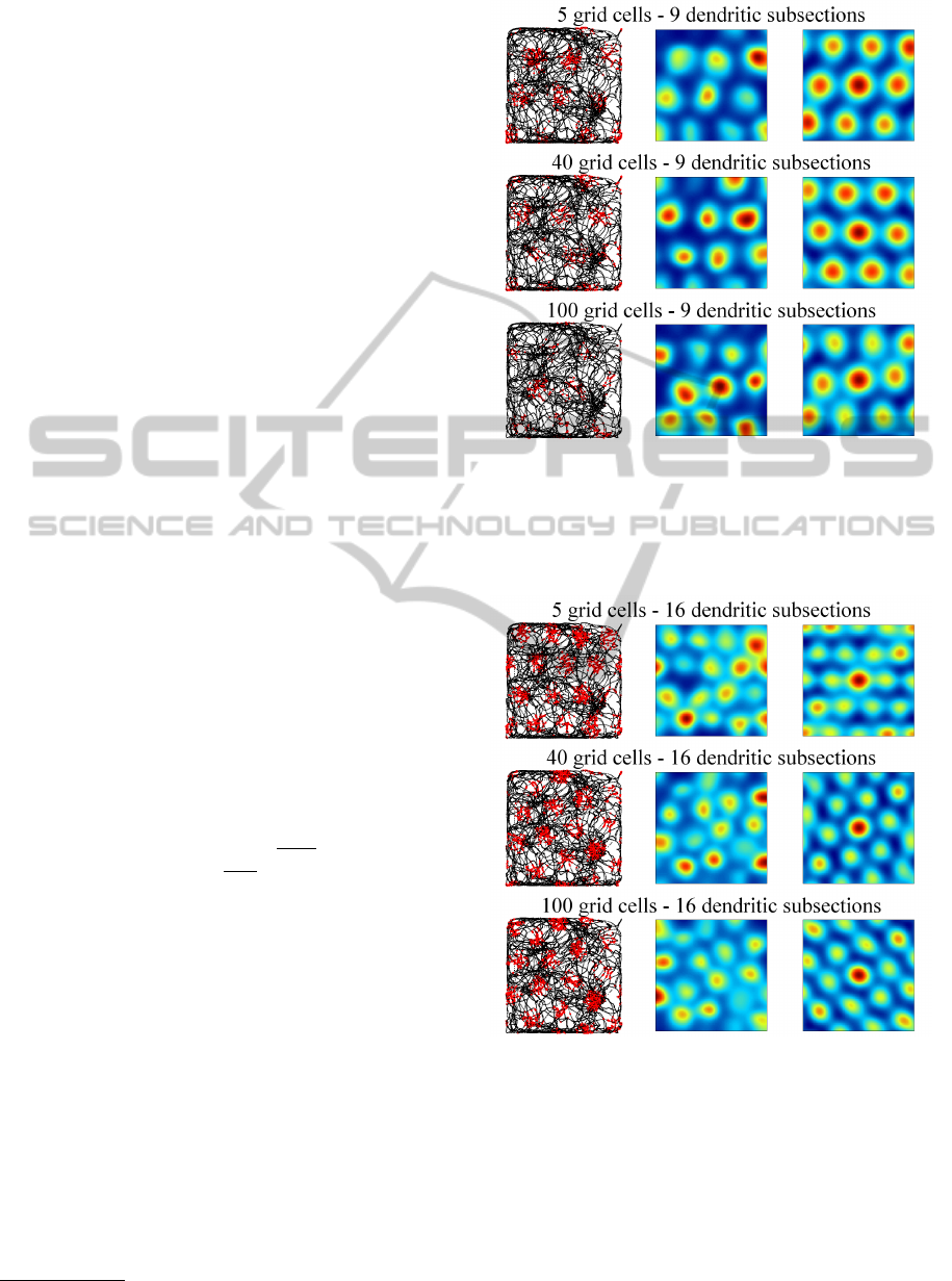
Figures 4, 5, and 6 illustrate the activity of indi-
vidual grid cells (rows) with 9 (fig. 4), 16 (fig. 5) and
25 (fig. 6) dendritic subsections in groups of 5, 40,
and 100 grid cells. The left column shows the path
of the rat (black lines) and simulated spikes of the
particular grid cell (red dots). The spikes were sim-
ulated with a gaussian probability propotional to the
grid cells activity a
g
. The middle column shows the
4
data is available at http://www.ntnu.no/cbm/gridcell
Figure 4: Each row shows the activation of a single, simu-
lated grid cell with 9 dendritic subsections in a group of 5,
40, and 100 grid cells. The left side shows the path of the rat
(black lines) and simulated spikes of the grid cell (red dots).
The right side shows the autocorrelogram (central portion)
of the grid cell’s rate map (middle column).
Figure 5: Activity of simulated grid cells with 16 dendritic
subsections in groups of 5, 40, and 100 grid cells. Illustra-
tion corresponding to figure 4.
averaged rate map of the grid cell and the right col-
umn shows the autocorrelogram of the rate map (blue
colors represent low values, red colors represent high
values). Both maps were generated according to the
methods proposed by (Sargolini et al., 2006). The fig-
ures illustrate that spacing and firing field size of the
simulated grid cells is only dependent on the number
IJCCI2013-InternationalJointConferenceonComputationalIntelligence
426
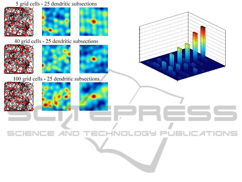
Figure 6: Activity of simulated grid cells with 25 dendritic
subsections in groups of 5, 40, and 100 grid cells. Illustra-
tion corresponding to figure 4.
of dendritic subsections, whereas the number of grid
cells per group has no influence. Well formed, trian-
gular firing patterns were achieved by grid cells with
9 and 16 dendritic subsections. Grid cells with 25 or
more (not shown) dendritic subsections did not yield
a proper triangular pattern. However, the spike map
still shows a regular, almost triangular firing pattern
that could in principle still serve as a means to encode
spatial information in a grid-like way.
Figure 7 illustrates the alignment process of grid
cell orientations on the network level. In the begin-
ning grid cell orientations cover the whole spectrum
of orientations in a 60 degree window with a slight
emphasis of the orientations around 20 and 30 de-
grees. Gradually over time the grid cells align their
orientations to a common orientation of about 30 de-
grees. The orientation of the grid cells was deter-
mined as proposed by (Sargolini et al., 2006).
A second set of experiments using 170 minutes of
rat movement data as input without an initial phase
of random inputs yielded similar results. However,
the learning rates had to be reduced by two orders of
magnitude to result in a stable formation of grid pat-
terns.
7 DISCUSSION
We presented a computational model of grid cells that
is capable to generate the peculiar, triangular firing
pattern observed in real grid cells and that provides an
time step
0
50
100
150
200
250
300
3
10×
angle
0
0.2
0.4
0.6
0.8
1
1.2
0
2
4
6
8
10
12
14
16
18
development of grid orientation
Figure 7: Development of grid cell orientation within
300.000 time steps. The group of 20 grid cells gradually
aligns their orientations to a common value of about 30 de-
grees.
explanation how a group of grid cells can align their
orientations with a self-organizing process on a net-
work level. In addition to this, the model facilitates
plausible argumentations to account for other proper-
ties of grid cells reported in section 3:
• Although spacing and orientation of co-localized
grid cells are similar, they typically differ in their
phase. This is also true for the presented model as
the phase of a model grid cell is predominantly de-
termined by the random, initial conditions of the
first two dendritic subsections. The connections
made to other grid cells on the network level are
activity-based and not location-based.
• The entorhinal cortex contains discrete grid cell
modules that have separate and distinct grid spac-
ings. In the current model, the grid spacing can be
influenced by the number of dendritic subsections
or by the level of speed modulation of the two
one-dimensional attractor-networks that generate
the orthogonal, periodic input to our grid cells.
• The sudden realignment of the grid orientation
and phase when an animal enters a new environ-
ment can be explained on the input level. A re-
alignment of the head-direction cells affects im-
mediately the four neurons that approximate the
sine and cosine fractions effectively rotating the
coordinate system of the model grid cells.
• The reported increase in the size of grid cells
could reflect a change in the speed modulation
of the two input attractor networks. If, e.g., the
speed signal is in part determined by some form
of optical flow and in part determined by internal,
self-motion signals, a new environment may re-
AComputationalModelofGridCellsbasedonDendriticSelf-organizedLearning
427

quire some adjustment before optical flow and in-
ternal self-motion signals produce a coherent sig-
nal again.
• Grid cells which are already present in a coarse
and rudimentary form in young rats even before
they start exploring their environment can be ex-
plained by random position inputs generated dur-
ing development.
Irrespective of these specific aspects regarding grid
cells the idea of a dendritic self-organizing map has
itself some intriguing consequences. Commonly, the
units of a self-organizing map (SOM) represent sin-
gle classes. In order to increase the “resolution” of a
SOM more units must be added. But the more units
are present in a SOM, the less inputs will be directed
towards each individual unit. As fewer and fewer in-
puts reach individual units, learning of new inputs be-
comes increasingly difficult. Additionally, if the in-
put is high-dimensional, the “curse of dimensional-
ity” will lead to a weak discrimination between the
individual units of the SOM. This contrasts the way
how grid cells encode information. Instead of repre-
senting a single region of the input space they sample
the whole input space at regular intervals, thus repre-
senting many regions, i.e., many classes, at once. In
order to identify a specific region of the input space,
grid cells of different groups with different orienta-
tion and spacing form a population code that uniquely
identifies the particular region. As each cell has only
a few units, i.e., dendritic subsections, in their local
SOM they suffer less from the curse of dimensional-
ity. Furthermore, a grid cell encoding of information
may be metabolically more efficient than the encod-
ing represented by a common SOM. Grid cells cover
the whole input space and are to that effect more fre-
quently active than cells of a SOM which may be only
rarely used but have to be maintained anyway.
8 CONCLUSIONS AND
OUTLOOK
We have presented a plausible computational model
of grid cells using a dendritic self-organizing map as
one of its core components. The model is not only
able to generate the peculiar, triangular firing pattern
of grid cells, but is also able to provide plausible ar-
guments that can account for several other phenomena
observed in the context of grid cells.
We argue that the way how grid cells encode spa-
tial information may represent a more general con-
cept of how high-level information is processed in the
brain. It appears promising to investigate how other
input modalities can be represented by a population
code of dendritic SOMs. These modalities include
high level feature descriptions of images, sound or
more abstract signals like the posture of the body.
REFERENCES
Barry, C., Ginzberg, L. L., OKeefe, J., and Burgess, N.
(2012). Grid cell firing patterns signal environmen-
tal novelty by expansion. Proceedings of the National
Academy of Sciences, 109(43):17687–17692.
Burgess, N., Barry, C., and O’Keefe, J. (2007). An oscilla-
tory interference model of grid cell firing. Hippocam-
pus, 17(9):801–812.
Derdikman, D., Whitlock, J. R., Tsao, A., Fyhn, M., Haft-
ing, T., Moser, M.-B., and Moser, E. I. (2009). Frag-
mentation of grid cell maps in a multicompartment en-
vironment. Nat Neurosci, 12(10):1325–1332.
Fiete, I. R., Burak, Y., and Brookings, T. (2008). What
grid cells convey about rat location. The Journal of
Neuroscience, 28(27):6858–6871.
Fritzke, B. (1995). A growing neural gas network learns
topologies. In Advances in Neural Information Pro-
cessing Systems 7, pages 625–632. MIT Press.
Fuhs, M. C. and Touretzky, D. S. (2006). A spin glass model
of path integration in rat medial entorhinal cortex. The
Journal of Neuroscience, 26(16):4266–4276.
Fyhn, M., Hafting, T., Treves, A., Moser, M.-B., and
Moser, E. I. (2007). Hippocampal remapping and
grid realignment in entorhinal cortex. Nature,
446(7132):190–194.
Fyhn, M., Molden, S., Witter, M. P., Moser, E. I., and
Moser, M.-B. (2004). Spatial representation in the en-
torhinal cortex. Science, 305(5688):1258–1264.
Giocomo, L., Moser, M.-B., and Moser, E. (2011). Com-
putational models of grid cells. Neuron, 71(4):589 –
603.
Hafting, T., Fyhn, M., Molden, S., Moser, M.-B., and
Moser, E. I. (2005). Microstructure of a spatial map
in the entorhinal cortex. Nature, 436(7052):801–806.
Kropff, E. and Treves, A. (2008). The emergence of grid
cells: Intelligent design or just adaptation? Hip-
pocampus, 18(12):1256–1269.
Langston, R. F., Ainge, J. A., Couey, J. J., Canto, C. B.,
Bjerknes, T. L., Witter, M. P., Moser, E. I., and Moser,
M.-B. (2010). Development of the spatial representa-
tion system in the rat. Science, 328(5985):1576–1580.
McNaughton, B. L., Battaglia, F. P., Jensen, O., Moser, E. I.,
and Moser, M.-B. (2006). Path integration and the
neural basis of the ’cognitive map’. Nat Rev Neurosci,
7(8):663–678.
Mhatre, H., Gorchetchnikov, A., and Grossberg, S. (2012).
Grid cell hexagonal patterns formed by fast self-
organized learning within entorhinal cortex. Hip-
pocampus, 22(2):320–334.
Monaco, J. D. and Abbott, L. F. (2011). Modular realign-
ment of entorhinal grid cell activity as a basis for hip-
pocampal remapping. The Journal of Neuroscience,
31(25):9414–9425.
IJCCI2013-InternationalJointConferenceonComputationalIntelligence
428

Moser, E. I., Kropff, E., and Moser, M.-B. (2008). Place
cells, grid cells, and the brain’s spatial representation
system. ANNUAL REVIEW OF NEUROSCIENCE,
31:69–89.
Navratilova, Z., Giocomo, L. M., Fellous, J.-M., Hasselmo,
M. E., and McNaughton, B. L. (2012). Phase preces-
sion and variable spatial scaling in a periodic attractor
map model of medial entorhinal grid cells with real-
istic after-spike dynamics. Hippocampus, 22(4):772–
789.
O’Keefe, J. (1976). Place units in the hippocampus of the
freely moving rat. Experimental Neurology, 51(1):78
– 109.
O’Keefe, J. and Dostrovsky, J. (1971). The hippocampus as
a spatial map. preliminary evidence from unit activity
in the freely-moving rat. Brain Research, 34(1):171 –
175.
Sargolini, F., Fyhn, M., Hafting, T., McNaughton, B. L.,
Witter, M. P., Moser, M.-B., and Moser, E. I.
(2006). Conjunctive representation of position, di-
rection, and velocity in entorhinal cortex. Science,
312(5774):758–762.
Sjstrm, P. J., Rancz, E. A., Roth, A., and Husser, M. (2008).
Dendritic excitability and synaptic plasticity. Physio-
logical Reviews, 88(2):769–840.
Solstad, T., Boccara, C. N., Kropff, E., Moser, M.-B.,
and Moser, E. I. (2008). Representation of geo-
metric borders in the entorhinal cortex. Science,
322(5909):1865–1868.
Squire, L., Bloom, F., Spitzer, N., Squire, L., Berg, D.,
du Lac, S., and Ghosh, A. (2008). Fundamental Neu-
roscience. Fundamental Neuroscience Series. Elsevier
Science.
Stensola, H., Stensola, T., Solstad, T., Froland, K., Moser,
M.-B., and Moser, E. I. (2012). The entorhinal grid
map is discretized. Nature, 492(7427):72–78.
Taube, J. (2009). Head direction cells. Scholarpedia,
4(12):1787.
Taube, J., Muller, R., and Ranck, J. (1990). Head-direction
cells recorded from the postsubiculum in freely mov-
ing rats. i. description and quantitative analysis. The
Journal of Neuroscience, 10(2):420–435.
van Strien, N. M., Cappaert, N. L. M., and Witter, M. P.
(2009). The anatomy of memory: an interactive
overview of the parahippocampal-hippocampal net-
work. Nat Rev Neurosci, 10(4):272–282.
Wills, T. J., Cacucci, F., Burgess, N., and O’Keefe, J.
(2010). Development of the hippocampal cognitive
map in preweanling rats. Science, 328(5985):1573–
1576.
Witter, M. P., Wouterlood, F. G., Naber, P. A., and van
Haeften, T. (2000). Anatomical organization of the
parahippocampal-hippocampal network. Annals of the
New York Academy of Sciences, 911(1):1–24.
Yartsev, M. M., Witter, M. P., and Ulanovsky, N. (2011).
Grid cells without theta oscillations in the entorhinal
cortex of bats. Nature, 479(7371):103–107.
Zilli, E. A. and Hasselmo, M. E. (2010). Coupled noisy
spiking neurons as velocity-controlled oscillators in a
model of grid cell spatial firing. The Journal of Neu-
roscience, 30(41):13850–13860.
AComputationalModelofGridCellsbasedonDendriticSelf-organizedLearning
429
