
Heart Rate Variability
Knowing More about HRV Analysis and Fatigue in Transport Studies
Jesús Murgoitio Larrauri
1
, José Luis Gutierrez Temiño
2
and María José Gil Larrea
2
1
Fundación Tecnalia Research & Innovation, Ibaizabal Bidea 202 - Parque Tecnológico de Bizkaia, Zamudio, Spain
2
ESIDE, University of Deusto, Avenida de las Universidades 24, Bilbao, Spain
Keywords: Heart Rate Variability, HRV, Fatigue, Transport Applications.
Abstract: The use of ECG signal and derived HRV (Heart Rate Variability) analysis is a well-known technique for
detecting different levels of fatigue for objective evaluation in human activities (e.g. car-driver state
monitoring). This work takes a step further in detecting the first signals of fatigue without any hard methods
(usually car-drivers are forced not to rest for many hours). So, based on data coming from the ECG signal
for 24 experiments and the same number of different car-drivers driving for 3 hours starting in good
conditions, some correlations between fatigue and heart physiology has been explored through data mining
methods. Finally, one classifier based on a particular entropy evaluation has been used due to its very good
behaviour (True-Positives > 75 % and ROC area > 90 %). This work, using not the classifier itself but its
behaviour when the parameter known as “blending” (“blending” defines a different “neighbour” concept) is
changed, shows how the entropy between the computed “five minutes” driving windows (each window is
defined by a group of 15 previously selected variables) is more independent of the neighbour when these
time-windows are near to two hours driving. The work concludes that the entropy is more stable when
drivers reach two hours driving and this way will be promising. Consequently, it is proposed further studies
in the future based on this entropy concept too, but now integrating additional factors, e.g. age and circadian
cycles, which can complete and improve the HRV analysis, including different scenarios or applications out
of the safety in the transport studies.
1 INTRODUCTION
All studies about drivers state monitoring agree on
the detection of the first signals of fatigue around the
second hour driving. This is the reason why many
driving associations and public authorities
recommend taking a rest at least every two hours
driving. The figure 1 (RACE, 2011) obtained from
the 2011 report about fatigue is an example and
shows once again this aspect.
Thus, trying to find an objective method based
on physiological activity which is easy to use in
driving experiments when drivers drive a car,
TECNALIA Research & Innovation and the
University of Deusto has been working on using
ECG signal mainly focused on detection of the first
signals of fatigue. Furthermore, the reason for
considering it to be of interest to integrate the driver
ECG signal within the car system is closely related
to the “driver mental workload” measurement and
the relation with some physiological indices.
Figure 1: Evolution of the risk of fatigue when driving
(RACE).
Furthermore, most of the studies about driver
monitoring using ECG signal analyse this
information through the HRV (Heart Rate
Variability) but force drivers not to sleep for hours.
These previous experiences showed the influence of
fatigue in heart activity but it is not the most real
situation because the usual scenario is to start
driving in normal conditions. Besides, the part of
information coming from the ECG signal and
closely related to fatigue is very low and is
frequently only detected when fatigue is really
107
Murgoitio Larrauri J., Gutierrez Temiño J. and Gil Larrea M..
Heart Rate Variability - Knowing More about HRV Analysis and Fatigue in Transport Studies.
DOI: 10.5220/0004666501070114
In Proceedings of the International Congress on Cardiovascular Technologies (IWoPE-2013), pages 107-114
ISBN: 978-989-8565-78-5
Copyright
c
2013 SCITEPRESS (Science and Technology Publications, Lda.)

evident or high. On the other hand it is clear that
other physiological signals like EEG are better but
more difficult to analyse and need more expensive
devices and methods.
In the following lines we will introduce you to
the reasons why only a small part of the data coming
from the heart activity has information we are
interested in.
1.1 Heart Activity
Two anatomically different structures are used as
physiological indicators of workload measures:
Central Nervous System (CNS, it includes the brain,
brain stem, and spinal cord cells), and Peripheral
Nervous System (PNS) measures. The PNS can be
divided into the Somatic Nervous System (SoNS,
concerned with the activation of voluntary muscles)
and Autonomic Nervous System (AuNS, controls
internal organs and is autonomous because AuNS
innervated muscles are not under voluntary control).
The AuNS is further subdivided into the
Parasympathetic Nervous System (PaNS, to
maintain bodily functions) and the Sympathetic
Nervous System (SyNS, for emergency reactions):
Figure 2: Anatomical structures.
Most organs are dually innervated both by SyNS
and PaNS, and both can be coactive, reciprocally
active, or independently active. Heart rate is an
example of AuNS measures. So, the heart is
innervated both by the PaNS and SyNS. Each heart
contraction is produced by electrical impulses that
can be measured in the form of the ECG
(Electrocardiogram). The following figure shows the
well-known and typical register of heart electrical
activity:
Figure 3: Heart electrical activity.
Based on the information coming from this heart
electrical activity, time domain, frequency and
amplitude measures can be derived.
1.2 Time Domain
In the time domain usually the R-Waves of the ECG
are detected, and the time between these peaks (IBI:
Inter Beat Interval) is calculated. IBI is directly
related to Heart Rate (HR). However, this relation is
no linear and IBI is more normally distributed in
samples compared with HR. Thus, IBI scores should
be used for detection and testing of differences
between mean HR. IBI scales are less influenced by
trends than the HR scale.
According to some scientific works, average
heart rate during task performance compared to rest-
baseline measurement is a fairly accurate measure of
metabolic activity, and not only physical effort
affects heart rate level; emotional factors, such high
responsibility or the fear of failing a test, also
influence mean heart rate.
In the time domain, HRV is also used as a
measure of mental load. HRV provides additional
information to average HR about the feedback
between the cardiovascular systems and CNS
structures. In general HRV decrease is more
sensitive to increases in workload than HR increase.
Some works showed that an increase in physical
load decreased HRV and increased HR, while an
increase in mental load was accompanied by a
reduced HRV and no effect on HR (Lee and Park,
1990). Fatigue is reported to increase HRV
(Mascord and Heath, 1992) while low amounts of
alcohol decrease HRV (González González et al.,
1992).
1.3 Frequency Domain
In frequency domain, HRV is decomposed into
components that are associated with biological
control mechanisms (Kramer, 1991); (Porges and
Byrne, 1992). Three frequency bands have been
identified (Mulder, 1988; 1992): a low frequency
band (0.02-0.06 Hz) believed to be related to the
regulation of the body temperature, a mid frequency
band (0.07-0.14 Hz) related to the short term blood-
pressure regulation and a high frequency band (0.15-
0.50 Hz) believed to be influenced by respiratory-
related fluctuations (vagal, PaNS influenced –
(Kramer, 1991)):
CARDIOTECHNIX2013-InternationalCongressonCardiovascularTechnologies
108

Figure 4: HRV: frequency analysis (PSD=Power Spectral
Density, VLF= Very Low Frequencies, LF= Low
Frequencies, HF= High Frequencies).
A decrease in power in the mid frequency band
(“0,10 Hz” component) and in the high frequency
band have been shown to be related to mental effort
and task demands (Jorna, 1992); (Backs and Seljos,
1994); (Paas et al., 1994).
1.4 Amplitude Domain
Finally, amplitude information from the ECG signal
can be used to obtain information about workload.
The amplitude of the T-wave (TWA) is said to
mainly reflect SyNS (Furedy, 1996) and decreases
with increases in effort.
Driving is a very dynamic task in a changing
environment. Moreover, the driving task is large
influenced by drivers themselves. Nowadays, there
are factors that may even lead to increased human
failure in traffic:
The number of vehicles on the road is increasing,
so increased road intensity leads to higher
demands on the human information processing
system and an increased likelihood of vehicles
colliding.
People continue to drive well into old age.
Elderly people suffer from specific problems in
terms of divided attention performance, a task
that is more and more required in traffic. One of
the causes of these increased demands is the
introduction of new technology into the vehicle.
Drivers in a diminished state endanger safety on
the road (longer journeys, night time driving, and
so on). Driver fatigue is currently an important
factor in the cause of accidents.
The above mentioned factors and situations have
in common that in all cases driver workload is
affected. Although there are several definitions and
models to explain it, “mental workload” could be
defined as a relative concept; it would be the ratio of
demand to allocated resources. From this point of
view, several scientific works have demonstrated
that some parameters obtained from physiological
measures (pupil diameter, heart rate and respiratory,
electro dermal activity, EEG, electro-oculography
etc.) could help to ascertain the driver’s mental
workload and one of them is the ECG. Due to its
low level invasive characteristic, ECG information
seems very interesting information to increase safety
in driving tasks. The main idea is to use laboratory
methods considered in traffic research and based on
ECG signal.
From this point of view, as is explained in the
next section, several experiments have been carried
out to acquire data from ECG together with other
interesting information, but now focusing on
detecting specific patterns for the first signals of
fatigue around the second hour driving for normal
users in normal scenarios.
2 METHODS
In order to have significant data the methodology
followed can be structured in the following phases:
Experiments definition, data collection, and analysis.
The analysis includes one preliminary analysis for
classifier selection including attribute selection, and
a final analysis.
Anyway, although this work is focussed on the
HRV analysis and its application to the safety within
road transport scenarios, it can be considered as the
starting point to be extensible to any environment
related to the measurement of the working
conditions, e.g. other situations of risk of fatigue -
like working long-time periods in a hospital or in a
factory with a machine.
2.1 Experiment & Data Collection
Up to 24 experiments were carried out for 24
different drivers, all of them males and between 18
and 70 years old. Each driver was informed before
starting about it and the corresponding authorization
was also signed by them.
Every driver drove along one clear defined route
(always the same for every driver) completing
around three hours driving. The route had different
types of roads which were classified in five different
ways as is shown in the following table.
HeartRateVariability-KnowingMoreaboutHRVAnalysisandFatigueinTransportStudies
109
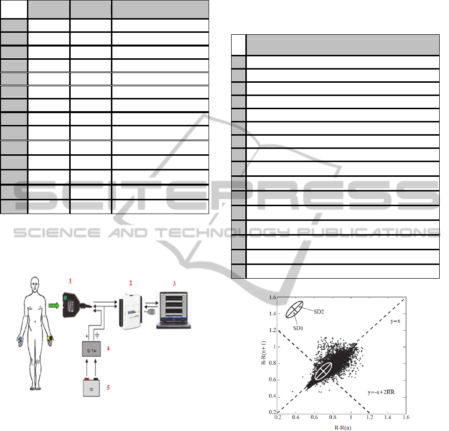
Table 1: Route description.
KM Code Type ofRoad
Start 0,0
0,5 C5 Urban
3,0 C1 Highway
44,0 C2 National (1 lane)
83,5 C1 Highway
97,1 C2 National (1 lane)
115,3 C3 Local
138,1 C4 Local - Mountain
151,5 C3 Local
158,0 C5 Urban
169,4 C1 Highway
210,0 C2 National (1 lane)
212,8 C1 Highway
End 213,3 C5 Urban
As the main information to be considered was
the ECG signal the following devices were designed
and used to collect ECG signal (three electrodes
based):
Figure 5: Three electrodes based ECG data acquisition
system (1=Amplifier, 2=NI USB 6009, 3=Laptop,
4=Regulator, 5=battery).
Additionally data such as distance and time for
each five minutes driving were collected too.
Finally, up to 41 parameters were considered and
computed to assign for each five-minutes windows
with 50 % overlapping, e.g. circadian cycle (M in
the morning and T in the afternoon), age, mean and
standard deviation of RR intervals, and the
following 16 parameters from the frequency domain
(see figure 4).
Additionally, based on the Poincaré plot (Kitlas,
2005) the following two measures were also
calculated in the time domain: SD1 (instantaneous
beat-to-beat variability of the data), SD2 (continuous
beat-to-beat variability). The ratio SD1/SD2 is used
as a measure of heart activity too.
Table 2: Frequency domain parameters.
Description
1 X coordinate of peak in VLF
2 Y coordinate of peak in VLF
3 X coordinate of peak in LF
4 Y coordinate of peak in LF
5 X coordinate of peak in HF
6 Y coordinate of peak in HF
7 X coordinate of centroid in VLF
8 Y coordinate of centroid in VLF
9 X coordinate of centroid in LF
10 Y coordinate of centroid in LF
11 X coordinate of centroid in HF
12 Y coordinate of centroid in HF
13 Area of VLF (PSD)
14 Area of LF (PSD)
15 Area of HF (PSD)
16 Ratio of LF/HF areas
Figure 6: Poincaré plot: SD1 & SD2 graphical.
So, SD1, SD2 and the corresponding ratio are
considered as some of the most summarized and
complete information about the heart no linear
behaviour.
2.2 Analysis
2.2.1 Classifier: Instance-based Learners
The task of classifying objects is one to which
researchers in artificial intelligence have devoted
much time and effort and many different approaches
CARDIOTECHNIX2013-InternationalCongressonCardiovascularTechnologies
110

have been tried with varying success. Some well-
known schemes and their representations include:
ID3 which uses decision trees (Quinlan, 1986),
FOIL which uses rules (Quinlan, 1990), PROTOS
which is a case-based classifier (Porter et al., 1990),
and the instance-based learners IB1-IB5 (Aha et al.,
1991); (Aha, 1992). These schemes have
demonstrated excellent classification accuracy over
a large range of domains.
In this work we will use the entropy as a distance
measure which provides a unified approach to
dealing with these problems. Specifically we will
use the K-Star (Cleary and Trigg, 1995), an
instance-based learner which uses such a measure.
Instance-based learners classify an instance by
comparing it to a database of pre-classified
examples. The fundamental assumption is that
similar instances will have similar classifications.
The question lies in how to define “similar instance”
and “similar classification”.
Nearest neighbour algorithms (Cover and Hart,
1967) are the simplest of instance-based learners.
They use certain domain specific distance functions
to retrieve the single most similar instance from the
training set. The classification of the retrieved
instance is given as the classification for the new
instance. Edited nearest neighbour algorithms (Hart,
1968); (Gates, 1972) are selective and in these
instances are stored in the database and used in
classification. The k nearest neighbours of the new
instance are retrieved and whichever class is
predominant amongst them is given as the new
instance's classification. A standard nearest
neighbour classification is the same as a k-nearest
neighbour classifier for which k=1.
One of the advantages of the approach we are
following here is that both real attributes and
symbolic attributes can be dealt with together within
the same framework.
For K-Star we have to choose values for the
blending parameter. The behaviour of the distance
measure as these parameters change is very
interesting. Consider the probability function for
symbolic attributes as “s” changes. With a value of
“s” close to 1, instances with a symbol different to
the current one will have a very low transformation
probability, while instances with the same symbol
will have a high transformation probability. Thus the
distance function will exhibit nearest neighbour
behaviour. As “s” approaches 0, the transformation
probability directly reflects the probability
distribution of the symbols, thus favouring symbols
which occur more frequently. This behaviour is
similar to the default rule for many learning schemes
which is simply to take whichever classification is
most likely (regardless of the new instance's attribute
values). As “s” changes, the behaviour of the
function varies smoothly between these two
extremes. The distance measure for real valued
attributes exhibits the same properties.
So, the K-Star algorithm chooses a value for
“blending” (mentioned “s” parameter) by selecting a
number between n0 and N. Thus selecting n0 gives a
nearest neighbour algorithm and choosing N gives
equally weighted instances. For convenience the
number is specified by using the “blending
parameter” b, which varies from b= 0% (for n0) and
b=100% for N, with intermediate values interpolated
linearly.
We think of the selected number as a “sphere of
influence”, specifying how many of the neighbours
should be considered important (although there is
not a harsh cut off at the edge of the sphere—more
of a gradual decreasing in importance).
The underlying technique solves the smoothness
problem and we believe contributes strongly to its
good overall performance. The underlying theory
also allows clean integration of both symbolic and
real valued attributes and a principled way of
dealing with missing values (in this case symbolic
attributes were used).
2.2.2 Attribute Selection
For attribute selection, all five minutes windows
were labelled to defined six groups: “A” for the first
30 minutes driving, “B” for the next 30 minutes, and
so on until “F” for the last 30 minutes.
So, based on the WEKA (Waikato Environment
for Knowledge Analysis, version 3.6.6) tool and the
previously mentioned K-Star classifier, 15
parameters are shown to have the best confusion
matrix to classify all five minutes windows:
Figure 7: Confusion matrix.
The following figure shows the summary and the
detailed accuracy for each group, using “10-fold
cross validation” method for validation:
HeartRateVariability-KnowingMoreaboutHRVAnalysisandFatigueinTransportStudies
111
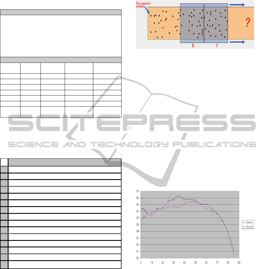
Table 3: Summary and Detailed Accuracy by class.
=== Summary ===
Correctly Classified Instances: 1.391 (78,3662 %)
Incorrectly Classified Instances: 384 (21,6338)
Kappa statistic: 0,7374
Mean absolute error: 0,0923
Root mean squared error: 0,235
Relative absolute error: 33,5625 %
Root relative squared error: 63,3865 %
Total Number of Instances: 1.775
=== Detailed Accuracy By Class ===
TP
Rate
FP
Rate
Precision ROC Area Class
0,792 0,031 0,841 0,963 A
0,824 0,056 0,771 0,958 B
0,836 0,058 0,767 0,955 C
0,752 0,052 0,768 0,939 D
0,755 0,047 0,785 0,938 E
0,694 0,018 0,773 0,958 F
0,784 0,047 0,785 0,951
Weighted
Avg.
The 15 parameters finally selected (assigned to
each five minutes window) to go further on the final
analysis were the following:
Table 4: Parameters selected.
Description
1 Circadian cycle (M=morning/T=afternoon)
2 Standard deviation of RR intervals (ms)
3 Mean of RR intervals (ms)
4 X coordinate of peak in LF (Hz)
5 X coordinate of peak in HF (Hz)
6 % of PSD for VLF
7 % of PSD for LF
8 % of PSD for HF
9 SD1: Improved standard deviation
10 SD2: Improved standard deviation
11 Ratio of PSD between LF/HF
12 X coordinate of centroid in VLF
13 X coordinate of centroid in LF
14 X coordinate of centroid in HF
15 Label of section in the route (A, B, C, D, E, F)
2.2.3 Final Analysis
Based on the preliminary analysis and results, a new
study was carried out considering only sections B
and C (each section = 30 minutes) when the border
between B and C sections was moved 5 to 5
minutes. It is graphically shown in the following
figure where each “dot” represents each of the five
minutes driving for one driver defined by the values
for the 15 parameters mentioned previously:
Figure 8: Two closed “30 minutes” windows moving
along the time.
Thus, the K-Star classifier behaviour to classify
B and C sections for different “blending”
(neighbour) values was analyzed for the border fixed
in each of the “t” instant.
3 RESULTS
The following figure shows this behaviour for two
different borders (series 1 and series 2) defined in
the route when the blending parameter is going from
0 to 100 %. It means that K-Star classifier behaviour
for “series 1” is improving from blending = 0 to 35
(until 89,3 % of correctly classified instances) and
then starts losing accuracy. So, this behaviour was
analyzed for different borders defined from 100
minutes to 135 all around the 2 hours (120 minutes):
Figure 9: Behaviour of the K-Star classifier for different
“blending” values (X=“blending”, Y=”accuracy”).
The final analysis of the behaviour of K-Star
classifier for each of the previously defined borders
(100-135) when the blending is changing showed
very interesting results about the entropy when the
first signals of fatigue are starting. It is graphically
documented in the following figure where e.g.
“Series 120” means the K-Star behaviour when the
border between B and C sections is defined in 120
minutes of the overall route. This analysis was
focused only on blending values between 15 % and
55 %, when the accuracy is the best and more stable.
CARDIOTECHNIX2013-InternationalCongressonCardiovascularTechnologies
112
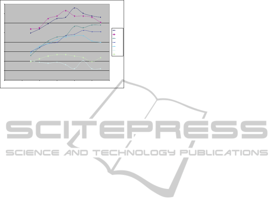
Figure 10: Behavior of the K-Star classifier during
different moments near the second hour guiding
(X=“blending”, Y=”accuracy”).
The conclusion, based on the above results over
24 drivers driving during three hours, is that the
entropy starts being more stable (classification is not
significantly better) at around the two hours driving
point while the neighbourhood (blending) changes
from 15 to 55 %. It could be explained because the
five minutes windows defined by the selected 15
parameters are more equally distributed and the
variability is decreasing when the first phase of
fatigue appears. This would be because the heart
variability starts losing elasticity (decreasing of
general alertness due to fatigue).
In any case, as is shown in the above figure,
some changes are detected through the entropy
analysis based on several time and frequency
domain parameters derived from the heart rate
variability (HRV) near to the first 120 minutes
driving.
4 DISCUSSION
The analysis of the entropy behaviour based on data
derived from the heart activity is a promising way to
detect first signals of different human factors (e.g.
fatigue, alertness etc.) which would be related to
some physiological mechanisms.
This entropy should be analyzed further to know
how different factors can influence it, i.e. how does
the age of the drivers affect the defined entropy
concept? Is it affected in the same way for women
and men? What about the behaviour during different
weather conditions? And the road type, related to the
different alertness levels needed to drive the car, is it
really better detected by the entropy within the HRV
behaviour? How much is the circadian cycle
influencing the heart activity and then the HRV?
Could the distance function of the “instances based”
classifier be improved in order to optimize and
detect the first signals of fatigue?
Since the entropy analysis of heart physiology
and HRV has been so promising, more questions
have appeared motivating us to go further in the
research carried out up to now, mainly oriented to
know better the physiology of the heart, and
correlative effects on some human behaviour.
Besides, although the results obtained has been
focussed on the safety in road transport scenarios,
this specific HRV analysis is the appropriate starting
point to be applied for the measurement of the
working conditions, i.e. different situations where
the risk of fatigue exists (long-time periods working
in a hospital or in a factory with a machine,…).
ACKNOWLEDGEMENTS
The authors wish to express their gratitude to the
group of researchers of the Transport unit in
TECNALIA Research & Innovation. Deepest
gratitude is also due to the support of Prof. Dr.
Dionisio Del Pozo Rojo and Prof. Dr. Jesús María
López González whose were extremely helpful and
offered invaluable assistance and guidance.
The authors would also like to convey thanks to
the Spanish Ministry of Industry, Tourism and
Commerce for providing the financial means and
ESIDE Faculty of University of Deusto (Bilbao) for
laboratory facilities.
REFERENCES
Aha, D. W., Kibler, D. & Albert, M. K. (1991) "Instance-
based Learning Algorithms." Machine Learning 6, pp.
37-66.
Aha, D. W. (1992) “Tolerating Noisy, Irrelevant and
Novel Attributes in Instance-based Learning
Algorithms.” International Journal of Man Machine
Studies 36, pp. 267-287.
Backs, R. W.; Seljos, K. A. (1994). Metabolic and cardio
respiratory measures of mental effort: the effects of
level of difficulty in a working memory task.
International journal of Psychophysiology, 16, 57-68.
Cleary John G., Trigg Leonard E (1995). “K*: An
Instance-based Learner Using an Entropic Distance
Measure”. 12th International Conference on Machine
Learning.
Cover, T. T. & Hart, P. E. (1967) "Nearest Neighbour
Pattern Classification." IEEE Transactions on
Information Theory 13, pp. 21-27.
Furedy, J.; Szabo A.; Péronnet, F. (1996). Effects of
82
83
84
85
86
87
88
89
90
0 1020 30405060
Seri e 10
0
Seri e 10
5
Seri e 11
0
Seri e 12
0
Seri e 12
5
Seri e 13
0
Seri e 13
5
HeartRateVariability-KnowingMoreaboutHRVAnalysisandFatigueinTransportStudies
113

psychological and physiological challenges on heart
rate, T-wave amplitude, and pulse-transit time.
International Journal of Psychophysiology, vol 22,
173-183.
Gates, G. W. (1972) "The Reduced Nearest Neighbour
Rule." IEEE Transactions on Information Theory 18,
pp. 431-433.
González González, J.; Mendez Llorens, A.; Mendez
Novoa, A.; Cordero Valeriano, J. J. (1992) Effect of
acute alcohol ingestion short term heart rate
fluctuations. Journal of studies on Alcohol, 53, 86-90.
Hart, P. E. (1968) "The Condensed Nearest Neighbour
Rule." IEEE Transactions on Information Theory 14,
pp. 515-516.
Jorna, P. G. A. M. (1992). Spectral analysis of heart rate
and psychological state: a review of its validity as a
workload index. Biological Psychology, 34, 237-257.
Kitlas A., Oczeretko E., Kowalewski M., Urban M. (2005)
"Nonlinear dynamics methods in the analysis of the
heart rate variability". Roczniki Akademii Medycznej
w Bialymstoku-Vol.50, 2005 – Suppl. 2. Annales
Academiae Medicae Bialostocensis.
Kramer, A. F. (1991). Physiological metrics of mental
workload: a review of recent progress. In D. L. Damos
(Ed.), Multiple-task performance. (pp 279-328).
Lee, D. H.; Park, K. S. (1990). Multivariate analysis of
mental and physical load components in synus
arrhythmia scores. Ergonomics, 33, 35-47.
Mascord D. J.; Heath (1992). Behavioural and
physiological indices of fatigue in a visual tracking
task. Journal of safety research, 23, 19-25.
Mulder, L. J. M. (1988). Assessment of cardiovascular
reactivity by means of spectral analysis. PhD Thesis.
Groningen: University of Groningen.
Mulder, L. J. M. (1992). Measurement and analysis
methods of heart rate and respiration for use in applied
environments. Biological Psychology, 34, 205-236.
Paas, F. G. W. C.; Van Merrienboer, J. G. J; & Adam, J. J.
(1994). Measurement of cognitive load in instructional
research. Perceptual and motor skills, 79, 419-430.
Porges, S. W.; Byrnes, E. A. (1992). Research methods for
measurement of heart rate and respiration. Biological
Psychology, 34, 93-130.
Porter, B. W., Bareiss, R. & Holte, R. C. (1990) "Concept
Learning and Heuristic Classification in Weak-theory
Domains." Artificial Intelligence 45, pp. 229-263.
Quinlan, J. R. (1986) "Induction of Decision Trees."
Machine Learning 1, pp. 81-106.
Quinlan, J. R. (1990) "Learning Logical Definitions from
Relations." Machine Learning 5, pp 239-266.
RACE (Real Automóvil Club de España). (2011). Informe
2011: La fatiga en la conducción.
CARDIOTECHNIX2013-InternationalCongressonCardiovascularTechnologies
114
