ANALYSIS OF ELECTROMAGNETIC FIELDS IN
INHOMOGENEOUS MEDIA BY FOURIER SERIES EXPANSION
METHODS－THE CASE OF A DIELECTRIC CONSTANT MIXED
A POSITIVE AND NEGATIVE REGIONS
Tsuneki Yamasaki
1
1
Department of Electrical Engineering, College of Science and Technology, Nihon University
Keywords: Inhomogeneous and negative medium, Improved Fourier series expansion, Electromagnetic wave.
Abstract: In this paper, we propose a new method for the electromagnetic fields with inhomogeneous media mixed the
positive and negative regions which is the combination of improved Fourier series expansion method using
the extrapolation method. Numerical results are given for the power reflection and transmission coefficient,
the energy absorption, the electromagnetic fields, and the power flow in the inhomogeneous medium mixed
the positive and negative regions including the case when the permittivity profiles touches zero for the TM
wave. The results of our method are in good agreement with exact solution which is obtained by MMA.
1 INTRODUCTION
Recently, the scattering and guiding problems of the
inhomogeneous media have been of considerable
interest, such as optical fiber gratings , photonic
bandgap crystals , frequency selective devices, and a
negative medium(Caloz et al.,2004). In the negative
medium, such as a plasma (Freidberg et al.,1972) or
a metallic grating(Yasuura et al.,1986), the
permittivity has both positive and negative regions.
One of the methods that are commonly employed
in solving the problems in an inhomogeneous
medium is the homogeneous multilayer
approximation method (HMA). Although the
method is widely known and is proved to solve the
electromagnetic fields in inhomogeneous media, it
cannot be applied to the positive and negative
regions with oblique angle of incidences in TM
wave.
Yamaguchi and Hosono(Yamaguchi et al.,1982)
pointed out this difficulty and applied the modified
multilayer approximation method(MMA) to this
problem. However MMA cannot be applied to the
case when the permittivity profiles touches zero. In
this case, HMA cannot also obtaine the
electromagnetic fields even if the loss term of the
permittivity tends to zero.
In this paper, we propose a new method for the
electromagnetic fields with inhomogeneous media
mixed the positive and negative regions which is the
combination of improved Fourier series expansion
method(Yamasaki et al.,1984) using the
extrapolation method.
K.F.Casey(Casey ,1972) has presented a Fourier
series expansion method to get the rigorous solution
in inhomogeneous madia. However, they did not
present any numerical results for the sinusoidally
stratified plasma media whose permittivity had the
only positive region(Casey et al.,1969).
Numerical results are given for the power
reflection and transmission coefficient, the energy
absorption, the electromagnetic fields, and the power
flow in the inhomogeneous medium mixed the
positive and negative regions including the case
when the permittivity profiles touches zero for the
TM wave. The results of our method are in good
agreement with exact solution which is obtained by
MMA.
30
Yamasaki T.
ANALYSIS OF ELECTROMAGNETIC FIELDS IN INHOMOGENEOUS MEDIA BY FOURIER SERIES EXPANSION METHODSTHE CASE OF A DIELECTRIC CONSTANT MIXED A
POSITIVE AND NEGATIVE REGIONS.
DOI: 10.5220/0004784800300038
In Proceedings of the Second International Conference on Telecommunications and Remote Sensing (ICTRS 2013), pages 30-38
ISBN: 978-989-8565-57-0
Copyright
c
 2013 by SCITEPRESS – Science and Technology Publications, Lda. All rights reserved

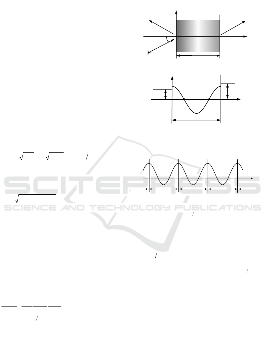
2 METHOD OF ANALYSIS
We consider an inhomogeneous medium mixed the
positive and negative regions as shown in Fig.1. The
structure is uniform in the y-direction and the
permittivity
2
()z
ε
has zero at
1
zz=
and
2
zz
=
(see Fig.1(b)) . The permeability is assumed to be
0
μ
. The time dependence is
exp( )it
ω
−
and
suppressed throughout.
In the formulation, the TM wave (the magnetic
field has only the y-component) is discussed. When
the TM wave is assumed to be incident from
0z
<
at the angle
0
θ
, the magnetic fields in the regions
1
(0)Sz≤
and
3
()Szd≥
are expressed(Yamasaki et
al.,1984) as
1
(0):Sz≤
()()
10 0 10 0
sin cos sin cos
(1)
,
ik x z ik x z
y
He Re
θθ θθ +−
=+ (1)
1100100
/, 2 ,kkk
ω
εμ ε ε π λ =
3
():Sz d≥
103
{sin ( )}
(3)
,
z
ikx k z d
y
HTe
θ +−
= (2)
22
3310
(sin)
x
kkk θ − ,
1, 3j
=
where
λ
is the wavelength in free space,
R
,and
T
are the reflection and transmission coefficient to
be determined by boundary conditions.
The inhomogeneous layer (
0 zd<<) consists of
periodically stratified layers which is the iteration of
the permittivity
2
()[ ()]
d
zz
ε
ε = in the original region
(
0 zd<<
;see Fig.2)( Yamasaki et al.,1984). The
modal component of magnetic field can be written
as
10
sin
(2)
()
ik x
y
HHze
θ
=
, and ()
H
z must satisfy the
following wave equation (Yamasaki et al.,1984
)
2
2
22
0010
()
() 1 ()
()
() ( sin ) () 0.
d
d
d
dz
dHz dHz
dz z dz dz
kz k Hz
ε
ε
εε θ
−
⎡⎤
+− =
⎣⎦
(3)
In the lossless case in
()
d
z
ε
, the singularity
appears in the second term in Eq.(3).
Taking into account the Floquet’s theorem,
()
H
z can
be approximated by the finite Fourier series as
2
()
N
ihz i nz d
n
nN
Hz e ue
π
=−
=
∑
(4)
To the obtain the correct solution in the analysis
of lossless case,
()
d
z
ε
is including the loss term
σ
(Yamasaki et al.,2004,2005(a),(b))
00
() ()/ ( 0).
d
d
zzi
ε
εε εσσ
+
≥

(5)
Substituting Eqs.(5) and (4) into Eq.(3), and
multiplying both side by
2
()
imzd
d
ze
π
ε
−

,and
rearranging after integrating with respect to
z in the
interval
0 zd
<
<
.We get the following equation in
regard to
h
(Yamasaki et al.,1984)
2
0,hh
+
+=MU CU KU
(6)
where
()
0
,,,
T
l
NN
uuu
−
⎡
⎤
⎣
⎦
U , :T transpose
,mn
η
⎡
⎤
⎣
⎦
M 
,
,mn
ζ
⎡
⎤
⎣
⎦
C 
,
,mn
γ
⎡⎤
⎣⎦
K 
,
,,
2
{2 ( )} },
nm nm
nnm
d
π
ζη
+−
0
θ
0
R
T
()i
y
H
1
S
2
S
3
S
(
)
10
,
ε
μ
()
30
,
ε
μ
(
)
20
(),z
ε
μ
d
x
z
(a) Coodinate system
d
0
z
1
ε
3
ε
1
z
2
z
2
()z
ε
(b)Distribution of dielectric constant
Fig.1 Structure of the inhomogeneous medium
mixed the positive and negative region.
z
()
d
zd
ε
−
(2)
d
zd
ε
−
()
d
z
ε
d
d
d
0
d
2d
3d
Fig 2. Periodically inhomogeneous layers
Analysis of Electromagnetic Fields in Inhomogeneous Media by Fourier Series Expansion Methods
31

2
22
,00,,
2
[(())(sin)] ,
nm nm nm
nnnm k
d
π
γθηξ
⎛⎞
+−+ −
⎜⎟
⎝⎠

(
)
,,,0,,mn N N=−  , (7)
{}
()
2
,0
0
1
()/
d
inmzp
nm d
ze dz
d
π
ηεε
−
∫


,
{}
()
2
2
2
0
,0
0
()/
d
inmzp
nm d
k
ze dz
d
π
ξεε
−
∫


.
Letting
hVU
and modifying Eq.(6), it is reduced
to the following conventional eigenvalue equation
,h=AW W
(8)
11−−
⎡⎤
⎢⎥
−−
⎣⎦
01
A
MK MC

,
⎡⎤
⎢⎥
⎣⎦
U
W
V

,
where 1 is unit vectore and M
-1
is inverse matrix of
M.
When it gets an eigenvalue
0
(;0)hi
β
αα =+ ≥
obtained Eq.(8) for
N →∞
,
0
()hi
β
α −=−−
is the
solution, and
0
(2/)hnd
π
±±
are also
solutions(Yamasaki et al.,1984
). Therefore we
selected
0
h
by convergence characteristics of
0
(2/)hnd
π
±±
in section of numerical analysis.
In the lossless case for
0
σ
→
, we can get the
eigenvalue
EV
h
according to the following
extrapolation equation
0EV
()ah
in regard to the
loss parameters
(13)
j
j
σ
= ～
(Yamasaki et
al.,2004,2005(a),(b))
2
0013
(); 1~3()
jjj
jhaaa σ
σ
σ ⋅+⋅ ==+ . (9)
In the same manner, the eigenvectors
(EV)
n
u
are
also obtained by the following extrapolation
equation (
(EV)
0 n
bu
) in regard to the loss
parameters
(13)
j
j
σ
= ～
(Yamasaki et
al.,2004,2005(a),(b))
() 2
01 3
(); 1~3()
EV
nj j j
bjubb σ
σ
σ ⋅+⋅ ==+
(10)
2
(0 ) :Szd<<
Using
E
V
h and
E
V
h− , and the corresponding
eigenvectors
(EV)
n
u
and
(-EV)
n
u
, the electromagnetic
fields in the inhomogeneous layer
(0 )zd<< are
expanded by a finite Fourier series(Yamasaki et al.,
2004, 2005(a),(b))
()
10
sin
(2) (2) (2)
()
[() ()],
EV
EV
ih z
ik x ih z
yEVEN
He tefzre f z
θ
νν
−
−
−
=+
(11)
()
2
() ,
N
EV
EV n
nN
n
iz
d
fz ue
π
=−
∑

()
()
2
() ,
N
EV
EV n
nN
n
iz
d
fz ue
π
−
−
=−
∑

{}
1
(2) (2)
() ,
xy
E
iz H z ωε
−
=
−∂∂
(12)
0 100 200 300 400
0.25
0.3
0.35
0.4
ν
2
d
β
π
2
d
α
π
2d
β
π
2d
α
π
Exac t Sol ut ion
0
100
30
N
θ
=
=

(a)Sinusoidal Profile case
ν
2
d
β
π
2
d
α
π
2d
β
π
2d
α
π
0
100
30
N
θ
=
=

(b)Linear Profile case
Fig.4
22.d and d vs
β
παπν
z
d
2
0
()z
ε
ε
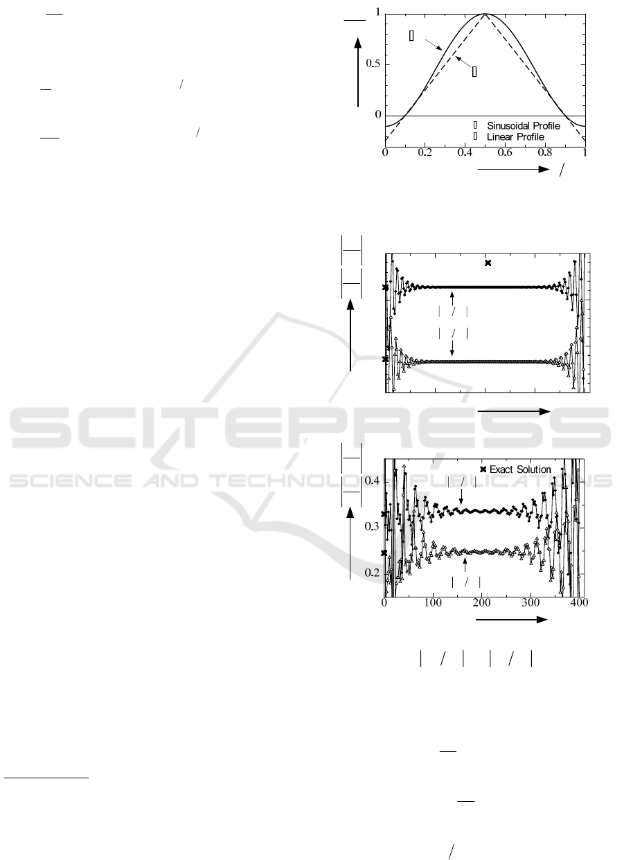
Fig.3 A profile of ① Eq.(15) and ② Eq.(16)
Second International Conference on Telecommunications and Remote Sensing
32

where,
(2)
t
ν
and
(2)
r
ν
are unknown coefficients which
satisfy the boundary conditions.
Using the boundary conditions and
()
E
V
TT=
can be
obtained by (the following equation):
() ()1,
EV EV
RNTN=−
()
( ) 2[ () ()]/( ),
EV EV
EV
TN dD dC ADCDff
−
=− −
(13)
where,
1
2
()
1
10
1
10
(0) ,
(0) ,
(0) cos
(0) cos
EV
EV
d
d
F
A
F
B
f
k
f
k
ε
εθ
ε
ε
θ
−
+
+


1
3
2
()
3
3
3
() ,
()
()
()
EV
EV
ih d
EV
x
ih d
EV
x
d
d
F
Cd e
F
Dd e
f
dk
f
dk
ε
ε
ε
ε
−
−
−
−


(14)
()
1
2
()
N
E
V
EV n
nN
n
Fhu
d
π
=−
+
∑

,
()
2
2
().
N
E
V
EV n
nN
n
Fhu
d
π
−
=−
−
∑

3 NUMERICAL ANALYSIS
We consider the following two profiles(see Fig.3):
(1)Sinusoidal profile:
20
()/ {1 cos(2 / )}
A
zzd
ε
εε δ π
=
− (15)
(2)Linear profile:
2
0
222
222
2
:0
()
2
2
(): 1
2
(min) [ (max) (min)]
(min) [ (max) (min )]
d
zz
z
d
d
zd z
d
ε
ε
ε
ε
εε
εε
⎡
<≤
⎢
=
⎢
⎢
−≤<
⎣
+−
+−
(16)
where,
σ
()
Re
EV
n
u
⎡⎤ ⎣⎦
200N =
100N =
50N =
0
30 θ =

(a)
()
Re
EV
n
u
⎡
⎤
⎣
⎦
σ
()
Im
EV
n
u
⎡⎤ ⎣⎦
200N =
100N =
50N =
0
30 θ =

(b)
()
Im
EV
n
u
⎡
⎤
⎣
⎦
Fig.6
() ()
Re Im .
EV EV
nn
u and u vs
σ
⎡⎤ ⎡⎤
⎣⎦ ⎣⎦
σ
2
d
β
π
200N =
100N =
50N =
0
30 θ =

(a)
2d
β
π
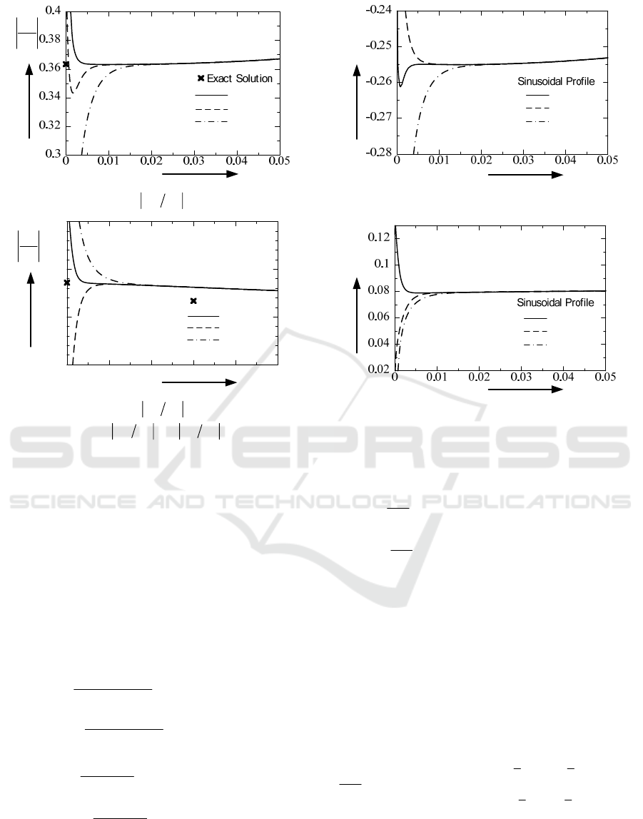
0 0.01 0.02 0.03 0.04 0.05
0.2
0.25
0.3
0.35
200N =
100N =
50N =
σ
2
d
α
π
Exact Solution
0
30 θ =

(b)
2d
α
π
Fig.5
22.d and d vs
β
παπσ
.
Analysis of Electromagnetic Fields in Inhomogeneous Media by Fourier Series Expansion Methods
33

22
22
22
,
2
,
[ (max) (min)]
[(max) (min)]
[ (max) (min)]
A
δ
ε
ε
ε
εε
εε
+
−
+


It has two zero points at
1
/ 0.0975zd≅ and
2
/0.9025zd≅
for both profiles. The values of
parameters chosen are
130
ε
εε ==
,
2
1(max)
ε
=
and
/0.8Ad λ = .
2
(min) 0.1
ε
=−
is the sinusoidal
case and
2
(min) 0.242236
ε
≅−
is the linear case.
Figures 4(a) and 4(b) show the convergence of
complex propagation constants
/(2 ) and /(2 )dd
β
παπ
to normalize
EV
()hi
β
α =+
with
100N
=
,
0.01
σ
=
,and
0
0
30
θ
=
for the mode number 12(2 1)N
ν
=+∼ .In
these Figures, cross points (×) are the exactsolution
which is obtained by the following characteristic
equation in regard to
h
(Hosono ,1973)
cos( ) ( )/2
SS
hd A D=+ , (17)
where,
and
SS
A
D
are the following Matrix
elements can be written using the Floquet’s theorem
(2) (2)
(2) (2)
0
(2)
(2)
SS
yy
SS
xx
z
zd
jhd
y
x
zd
AB
HH
CD
EE
H
e
E
=
=
=
⎡
⎤⎡⎤
⎡⎤
=
⎢
⎥⎢⎥
⎢⎥
⎣⎦
⎣
⎦⎣⎦
⎡⎤
=
⎢⎥
⎣⎦
∓
(18)
In Eq.(18),the magnetic fields
(2)
y
H
are expanded
by a finite power series(Budden ,1961)
which are
approximated by the linear profile including
2
() 0z
ε
=
as follows(Yamaguchi et al., 1982,
Budden ,1961):
10
sin
(2) (2) (2)
12
() ()
ik x
y
He twZrwZ
θ
νν
⎡
⎤
+
⎣
⎦

, (19)
where
2
2/3
0
2
02
()(),
()/
k
Z
z
dzdz
ε
εε
⋅
23
101
0
() ; 1, 0, ;
(2)
M
n
nn
nn
n
cb b
wZ aZ a a a
nn
−−
=
−
====
+
∑
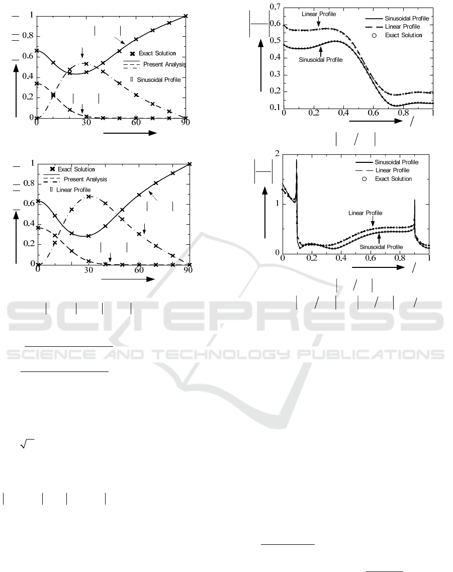
22
(), (),
EV EV
R
NTNG
2
()
EV
R
N
G
2
()
EV
TN
[
]
0
deg θ
}
(a) Sinusoidal Profile case
22
(), (),
EV EV
R
NTNG
2
()
EV
R
N
G
2
()
EV
TN
[
]
0
deg θ
}
(b) Linear Profile case
Fig.7
22
2
0
() () .
EV EV
R N and T N and G vs
θ
0
200
30
N
θ
=
=

z
d
(2)
()
y
i
y
H
H
(a)
(2) ( )i
yy
H
H
0
200
30
N
θ
=
=

z
d
(2)
()
x
i
x
E
E
(b)
(2) ( )i
x
x
E
E
Fig.8
(2) ( ) (2) ( )
.
ii
yy xx
H
H and E E vs z d
Second International Conference on Telecommunications and Remote Sensing
34

()
21 012
0
2
22 2
23
3
0002
() (log) () ; 1, 0, 0,
2
(1)
;sin/()/.
(2)
M
n
n
n
nn
n
c
wZ ZwZ bZ b b b
cb b c n
bckkdzdz
nn
θε
=
−−
=+===
−−−
==
−
∑
From Figure 4, the modal number chosen is
21N
ν
=+
(=201) gives good convergence in
comparison with the exact solution which is
obtained for
1000M =
in Eq.21. The values of exact
solution are
/(2 ) 0.3635d
β
π ≅
and
0.2859/(2 )d
α
π ≅
for the sinusoidal profile, and
/(2 ) 0.3303d
β
π ≅
and
0.2454/(2 )d
α
π ≅
for the
linear profile. The convergence tendency of the
sinusoidal profile is faster than that of the linear
profile. Figures 5(a) and 5(b) show the
/(2 )d
β
π
and
/(2 )d
α
π
for various values of loss term
σ
at
the modal number
(2 1)N
ν
=+ in the sinusoidal
profile. The results of the present method seem to be
difficult when
σ
tends to zero for increasing modal
truncation number
N
, but the true value can be
obtained by extrapolation method.
Figures 6(a) and 6(b) show the eigenvectors
(EV)
n
u
(
()
Re
EV
n
u
⎡
⎤
⎣
⎦
and
()
Im
EV
n
u
⎡
⎤
⎣
⎦
) for various values
of loss term
σ
at the same conditions as in Fig.5 for
the sinusoidal profile. From Figure 6, the true value
of the eigenvectors
(EV)
n
u
can be obtained by the
extrapolation method for
200N ≥
. On the other
hand, the case of linear profile, the convergence
tendency is slower than that of sinusoidal profile.
But the extrapolation method is also effective
for
200N ≥
.
Figures 7(a) and 7(b) show the power reflection
coefficient
2
|()|
EV
R
N
the power transmission
coefficient
2
|()|
EV
TN
, and the power loss of energy
difference
22
() ()][1
EV EV
NNGR T−−
for various
values of incident angle
0
θ
using the extrapolation
method to select the loss term at
1
0.01,
σ
=
2
0.02
σ
=
,and
3
0.03
σ
=
.The results of the
present method are in good agreement with those of
exact solutions. The relative error to the exact
S
zd
0
200
30
N
θ
=
=

(a) Poynting Vector
S
z
d
,Sx Sz
Sx
Sz
0
200
30
N
θ
=
=

(b) Poynting Vector
,Sx Sz
Fig .9 Poynting Vector of Sinusoidal Profile
S
z
d
0
200
30
N
θ
=
=

(a) Poynting Vector
S
0 0.2 0.4 0.6 0.8 1
-1
0
1
z
d
,Sx Sz
Sx
Sz
0
200
30
N
θ
=
=

Linear Profile
(b) Poynting Vector
,Sx Sz
Fig.10 Poynting Vector of Linear Profile
Analysis of Electromagnetic Fields in Inhomogeneous Media by Fourier Series Expansion Methods
35

solutions is about 0.02% for the sinusoidal profile
and 0.2% for the linear profile when the modal
truncation number chosen is
200N =
. From Figure
7, the energy absorption
G
is nonzero even if the
medium is lossless case.
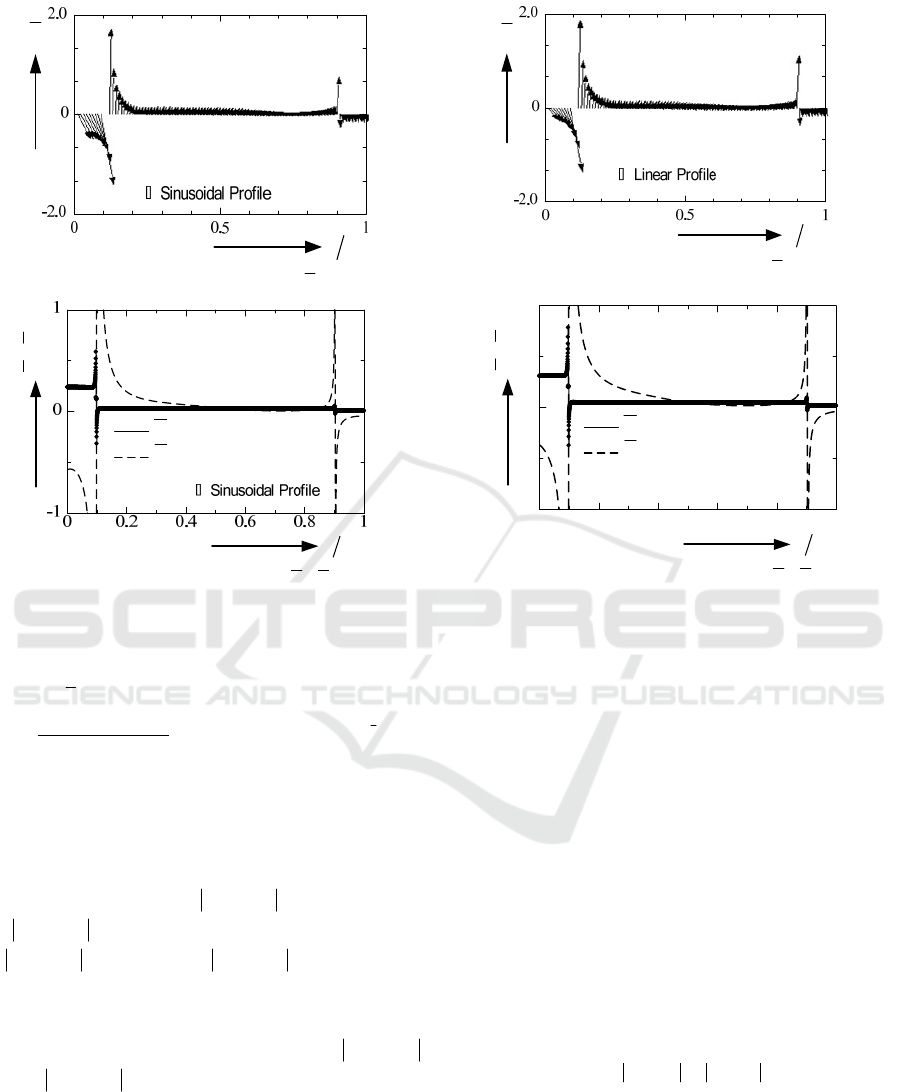
Figures 8(a) and 8(b) show the normalized
magnetic fields
(2) ( )
|/|
i
yy
HH
and the normalized
electric fields
(2) ( )
|/|
i
xx
E
E
for various values of
/zd
at
0
30 θ =

for
200N
=
using the extrapolation method in Fig.5
and Fig.6. From Fig.8, the results of the present
method are in good agreement with those of exact
solutions. In the sinusoidal case,
(2) ( )
|/|
i
yy
HH
is
about constant rather than that of the linear case in
0/0.4zd
≤
<
.This is attributed to the effect of the
profile and the angle of incidence
0
θ
.
On the other hand, the characteristic tendency of
(2) ( )
|/|
i
xx
E
E
is about same in both profiles, and the
effects of singularities are clearly seen at
1
/ 0.0975zd
≅
and
0.9025
, but it has the limited
value at this point because of
(2)
12
(or)/ 0
y
Hzzz∂∂=
,
1
(2) ( )
(2)
,
2
2
/
()/
lim .
()
()/
i
Exx
y
zzz
EE
H
zz
fz
dzdz
ε
→
∂
∂
=

(20)
In the Fig.8(b), the limiting values are
1
( ) 0.6096
E
fz
≅
and
2
( ) 0.4152
E
fz≅
.
Figures 9 and 10 show the Poynting vectors of
S
,
x
S
,and
z
S
for various values of
/zd
in the
inhomogeneous region with the same parameters as
in Fig.8 for both profiles. The definition of Poynting
vector is as follows:
,
xz
SS S=+i
j
Re 2,
Re 2.
x
zy
z
xy
SEH
SEH
∗
∗
⎡⎤
−×
⎣⎦
⎡⎤
×
⎣⎦


(21)
where,
i and
j
are unit vectors in the direction of
x
axis and
z
axis , respectively.
From Figs.9 and 10, we see the following
features:
(1)The effect of a positive and negative medium
are more significant at
1
/ 0.0975zd≅ and
2
/ 0.9025zd
≅
, so that the direction reverses to the
power flow
S
at that points.
(2) In the sinusoidal case,
z
S
has the limited
values at points of zeros
1
/ 0.0975zd≅
and
2
/ 0.9025zd
≅
, so that
1
( ) 0.1300
z
Sz≅
and
2
( ) 0.0166
z
Sz≅
, respectively.
On the other hand,
1
( ) 0.21245
z
Sz≅
and
2
( ) 0.03396
z
Sz≅
at those points for the linear case.
The energy of these points are absorbed.
zd
2
0
()z
ε
ε
Fig.11 A profile of ① Eq.(16) and ②Eq.(22)
z
d
(2)
()
y
i
y
H
H
(a)
(2) ( )i
yy
HH
(2)
()
x
i
x
E
E
(b)
(2) ( )i
x
x
E
E
Fig.12
(2) ( ) (2) ( )
and .
ii
yy xx
HH EEvszd
Second International Conference on Telecommunications and Remote Sensing
36

(3)
x
S
becomes infinite and the sign is reversed
at the singularities
1
/ 0.0975zd≅
and
2
/0.9025zd≅
.
In the investigation of above results, our methods
can be applied to the positive and negative medium
and have good accuracy of the electromagnetic
fields.
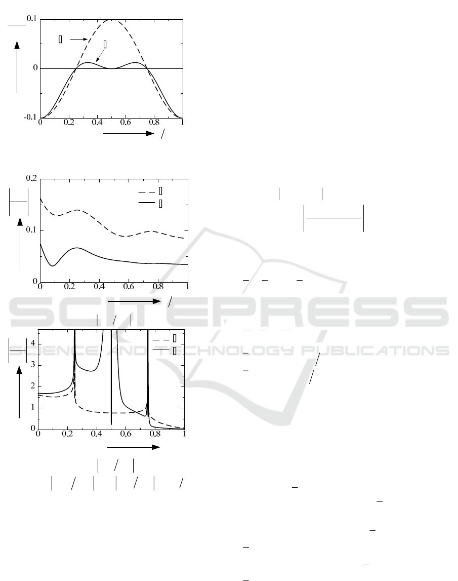
So, next we consider the distribution of permittivity
2
()z
ε
touches
2
() 0z
ε
= . This problem is difficult
to analyze by the MMA.
We consider the following sinusoidal profile②
(see Fig.(11))
20
()/ {0.5 cos(2 / )
0.5cos(4 / )}.
A
zzd
zd
ε
εε δ π
π
=−
+
(22)
It has three zero points at
1
/0.25zd
=
,
2
/0.5zd= ,and
3
/0.75zd=
. The definition of
A
ε
and
δ
are the same in Eq.(16). The values of
parameters chosen are
130
ε
εε ==
,
2
0.1(max)
ε
= (profile ① ),
2
0(max)
ε
= (profile
②) ,
2
(min) 0.1
ε
=−
and /0.8Ad λ = .
Figures 12(a) and 12(b) show the normalized
magnetic fields
(2) ( )
|/|
i
yy
HH
and the normalized
electric fields
(2) ( )
|/|
i
xx
E
E
for various values of
/zd
at
0
0
30 θ =
comparison with the profile ① in
Eq.(16) for
200N =
using the extrapolation
method .
From in Fig.(12), we see the following features:
(1)For the
(2) ( )
|/|
i
yy
HH
, the influence of distribution
of profiles ① and ② appears over
/0.5zd=
,
(2)The effect of the distribution of permittivity
2
()z
ε
which touches
2
() 0z
ε
= is more significant
of the electric fields
(2) ( )
|/|
i
xx
E
E
at
2
/0.5zd= , and
the limiting values are
1
( ) 3.2904
E
fz≅
,
2
( ) 0.35798
E
fz≅
and
3
( ) 0.65633
E
fz≅
for the profile
②. In the case of ①,there are
1
( ) 1.1417
E
fz≅
and
3
( ) 0.77027
E
fz
≅
.
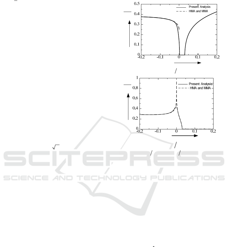
Finally, we investigate the complex propagation
constants in the periodically inhomogeneous layers
changing
20
(min) /
ε
ε
in the case of
fixed
20
(max)/ 1.0
ε
ε
=
in Eq.(16).
Figures 13(a) and 13(b) show the
/(2 )d
β
π
and
/(2 )d
α
π
for various values of
2
(min) 0.1 0.1
ε
=− ～
at
0
0
30 θ =
for
200N
=
using the extrapolation
method.
In this figure, the dashed line (---) are the results
of MMA (
2
(min) 0
ε
<
) and HMA (
2
(min) 0
ε
>
).
Both methods cannot be applied to the
2
(min) 0
ε
=
.
From in Fig.13, the results of MMA and HMA are
not accurate at
2
(min) 0
ε
=
,because the normalized
attenuation constant
/(2 )d
α
π
in this case appears
20
(min)/ 0.0295
ε
ε
≤
.
4 CONCLUSIONS
In this paper, The Fourier series expansion method is
applied to the electromagnetic fields with
inhomogeneous media mixed the positive and
negative regions using the extrapolation method
2
(min)
ε
2
d
β
π
0
200
30
N
θ
=
=

(a)
2d
β
π
2
(min)
ε
2
d
α
π
0
200
30
N
θ
=
=

(b)
2d
α
π
Fig.13
2
2and 2 . (min)ddvs
β
παπε
Analysis of Electromagnetic Fields in Inhomogeneous Media by Fourier Series Expansion Methods
37

which obtaines the correct value of the eigenvalue
and eigenvectors for the case of TM wave.
Numerical results are given for the power
reflection and transmission coefficient, the energy
absorption, the electromagnetic fields, and the power
flow in the inhomogeneous medium mixed the
positive and negative regions including the case of
the permittivity profiles touches zero for the case of
the TM wave. The results of our method are in good
agreement with exact solution which is obtained by
MMA.
REFERENCES
Budden K.C., 1961, Radio Waves in the Ionoshere,
Cambridge Univ., Press, pp.343-347.
Caloz C. , Itoh T.,2004, Microwave Application of
Metamaterial Structures, IEICE Technical Report.
Vol.104, No202, pp135-138.
Casey K.F., Matthes J.R. and Yeh C. ,1969, Wave
Propagation in Sinusoidally Stratified Plasma Media,
J.Math.Phys., Vol.10, no5, pp.891-896.
Casey K.F.,1972, Application of Hill’s Function to
problem of propagation in Stratified Media, IEEE
Tran.Antenas Propagt. ,vol.AP-20, 3, p.369-374.
Freidberg J.P., Mitchell R.W., Morse R.L. , Rudsinski
L.I.,1972,Resonant Absorption of Laser Light by Plasma
Targets, Phys. Rev. Lett.,Vol.28,no13.,pp.795-799.
Hosono T.,1973, Fundation of Electromagnetic Wave
Engineering, p.247, Shioko Publ. Co.(in Japanese) .
Yamaguchi S., Hosono T.,1982, Some Diffculties in
Homogeneous Multilayer Apporoximation Method and
Their Remedy, IEICE Trans.,Vol.J64-B, no10, pp.1115-
1122 (in Japanese 1981) [translated Scripta Technica,
INC., Vol.65-B, No.5 pp.75-83.
Yamasaki,T ,Hinata T.,Hosono H., 1984, Analysis of
Electrogagnetic Field in inhomogeneous Media by Foirier
Series Expansion Methods, IEICE Trans. Vol.J66-B,
no10., pp.1239-1246(in Japanese 1983) [translated Scripta
Technica, INC., Vol.67-B, No.6, pp.61-71.
Yamasaki t.,Isono K.,Hinata T., 2004, Analaysis of
Electromagnetic Field in Inhomogeneous media by
Fourier Series Expansion Method -The case of a dielectric
constant mixed in positive/negative medium , Part I ,IEE
Technical Reports Japan, EMT-04-121, pp.31-36(in
Japanese) .
Yamasaki t.,Isono K.,Hinata T., 2005(a), Analaysis of
Electromagnetic Field in Inhomogeneous media by
Fourier Series Expansion Method -The case of a dielectric
constant mixed in positive/negative medium, Part II, IEE
Technical Reports Japan, EMT-05-7, pp.35-40 (in
Japanese) .
Yamasaki T., Isono K., Hinata T., 2005(b), Analaysis
of Electromagnetic Fields in Inhomogeneous media by
Fourier Series Expansion Method -The case of a dielectric
constant mixed a positive and negative regions, IEICE
Trans. on Electronics, Vol.E88-C, No.12, pp.2216-2222.
Yasuura K., Murayama M., 1986, Numerical Analysis
of Diffraction from a Sinusoidal Metal Grating, IEICE
Trans.,Vol.J69-B, no2, pp.198-205 (in Japanese).
Second International Conference on Telecommunications and Remote Sensing
38