
SOUND SOURCE LOCALIZATION IN A SECURITY SYSTEM
USING A MICROPHONE ARRAY
Vera Behar
1
, Hristo Kabakchiev
2
and Ivan Garvanov
3
1
Institute of Information & Communication Technologie, BAS, 25-A Acad. G.Bonchev Str., Sofia, Bulgaria
2
Faculty of Mathematics & Informatics,Sofia University, 15 Tsar Osvoboditel Blvd., Sofia, Bulgaria
3
University of Library Studies & Information Technologies, Sofia, Bulgaria
behar@bas.bg, ckabakchiev@yahoo.com, igarvanov@yahoo.com
Keywords: Adaptive array processing, microphone arrays, sound signal processing, DOA estimation
Abstract: A possible algorithm for sound source localization in a security system that is based on
beamforming of a microphone array is described in this paper. It is shown that the adaptive
beamforming algorithm, Minimum Variance Distortionless Response (MVDR), can be a part of
the signal processing implemented in a security system. This signal processing includes the
following stages: sound source localization, signal parameter estimation, signal priority analysis
and, finally, control of protective and warning means (for example, video camera). The adaptive
beamforming method MVDR is used for estimating the direction-of arrival (DOA) of signals
generated by different sound sources, which arrive at the microphone array from different
directions of the protected area. The scenario, in which four sound sources located at different
points of the protected area generate different sound signals (warning, alarm, emergency and
natural noise), is simulated in order to verify the algorithm for DOA estimation. The simulation
results show that an adaptive microphone array can be successfully used for accurate localization
of all sound sources in the observation area. The parallel version of the described algorithm is
tested in Blue Gene environment using the interface MPI.
1 INTRODUCTION
The security system is a standard part of any
building in the city. In most sensors used by a
security system for protection of a limited space
(home, parking) are mounted sound sirens that are
activated in the event of an adverse situation in the
protected space. Usually, in case of such a situation
(fire, smoke, vibration, and breakage of glass or
opening the car) the sirens of sensors give a loud
beep for a few minutes. The assessment of the
direction and parameters of the incoming sound
signals can be used to control the movement of a
video camera that records the situation in the most
dangerous direction and submits the data to the
management centre.
The novelty of this paper is to use the adaptive
beamforming algorithm in order to locate, using a
microphone array, the direction of sound signals
coming from sensors or other sound sources.
Microphones arrays represent a set of microphones
arranged in some geometric configuration. They can
be realized as linear microphone arrays, where the
microphones are positioned in a straight line, or as
circular microphone arrays, where the microphones
are placed in a circle, or as rectangular microphone
arrays, where the microphones are arranged in the
shape of a rectangle plate (Benesty, 2008).
Microphone arrays have many advantages. Firstly,
the beamforming can be done digitally so as to
control all dangerous directions (door, windows,
cars) using only a single microphone array.
Otherwise, when using directional microphones of
other types, for example, parabolic microphones, a
lot of such microphones are required, because each
microphone can control only one direction.
Secondly, all noise signals coming from other
uncontrolled directions (speaking of people, banging
on the walls, etc.) are adaptively rejected by a
microphone array, which increases the detectability
of signals from sensors and improves the security of
the protected area. For comparison, when using a
85
Behar V., Kabakchiev H. and Garvanov I.
SOUND SOURCE LOCALIZATION IN A SECURITY SYSTEM USING A MICROPHONE ARRAY.
DOI: 10.5220/0004785700850094
In Proceedings of the Second International Conference on Telecommunications and Remote Sensing (ICTRS 2013), pages 85-94
ISBN: 978-989-8565-57-0
Copyright
c
2013 by SCITEPRESS – Science and Technology Publications, Lda. All rights reserved

directional parabolic microphone, noise signals are
not removed and they interfere with the detection of
the signal. In third, a microphone array can
simultaneously generate several independent beam
patterns and collect the information from multiple
sound sources. In the fourth, the signal power at the
output of a microphone array is increased M times
(M - is the number of array microphones), which
allows to substantially increase the security of the
protected area. Moreover, a three-dimensional area
can be controlled using the rectangular or circular
microphone arrays, and, finally, microphone arrays
can be easy adapted to detect acoustic signals with
different frequency characteristics by change of the
distance between microphones in the array.
In this paper, we propose to use the Minimum
Variance Distortionless Response (MVDR)
beamforming algorithm for DOA estimation of
signals arrived from different sound sources at a
microphone array (Godara, 1997; Trees, 2002;
Vouras, 1996; Moelker, 1996). We consider the
case, when each sound source is located in the
array’s far-field, and the sounds generated by sound
sources propagate through the air. The DOA is
proposed to be estimated as a direction, in which the
signal power at the output of a microphone array
exceeds a previously predetermined threshold. The
paper is structured as follows. In the next second
section, the expressions for calculation of array
response vectors are derived for three types of
microphone arrays. The model of signals arrived at a
microphone array in a security system is described
in the third section. The MVDR algorithm for DOA
estimation is mathematically described in the forth
section.
The parallel version of the MVDR algorithm
tested in Blue Gene environment using the interface
MPI is described in the fifth section. The simulation
scenario, in which four sound sources located at
different points of the protected area generate
different sound signals (warning, alarm, emergency
and natural noise), is described in the sixth section.
The simulation scenario is used in order to verify the
algorithm for DOA estimation. The results obtained
show that the MVDR beamforming algorithm
applied to a microphone array can be successfully
used for accurate localization of all sound sources in
the observation area. The parallel version of the
described algorithm is tested in Blue Gene
environment using the interface MPI.
2 MICROPHONE ARRAYS
Microphone arrays are composed of many
microphones working jointly to establish a unique
beam pattern in the desire direction. The array
microphones are put together in a known geometry,
which is usually uniform - Uniform Linear Arrays
(ULA), Uniform Rectangular Arrays (URA) or
Uniform Circular Arrays (UCA) (Ioannidis, 2005).
Since the ULA beam pattern can be controlled only
in one dimension (azimuth), so in various sound
applications, URA and UCA configurations with
the elements extended in two dimensions must be
used in order to control the beam pattern in two
dimensions (azimuth and elevation).
2.1 URA Configuration
In a URA array, all elements are extended in the x-y
plane. There are M
X
elements in the x-direction and
M
Y
elements in the y-direction creating an array of
(M
X
x M
Y
) elements. All elements are uniformly
spaced d apart in both directions. Such a rectangular
array can be viewed as M
Y
uniform linear arrays of
M
X
elements or M
X
uniform linear arrays of M
Y
elements. Usually, the first array element is
considered as the origin of Cartesian coordinates as
shown in Fig.1.
Figure 1: URA configuration
The direction of a signal arriving from azimuth φ
and elevation θ can be described with a unit vector e
in Cartesian coordinates as:
(1)
The vector r
m
in the direction of the m(i,k) element
can be described in Cartesian coordinates as:
(2)
Z
to a signal source
e
θ
Y
r
m
φ
X
Second International Conference on Telecommunications and Remote Sensing
86

Z
to a signal source
e
θ
1 Y
φ
1
r
1
φ
X
In (2), i and k denote the element position along the
y- and the x-axis, respectively. The sequential
element number m(i,k) is defined as:
(3)
If the first element in the rectangular array is a
reference element, the path-length difference d
m(i,k)
for a signal incident at element m(i,k) can be defined
as the projection of the vector r
m(i,k)
on the signal
direction vector e:
(4)
Therefore, the URA array response vector a
c
takes the form:
(5)
In (5), the total number of elements in the
microphone array is:
(6)
2.2 ULA Configuration
The ULA array response vector a
c
is calculated by
(5) where M
X
=1.
2.3 UCA Configuration
In a UCA array, all elements are arranged along the
ring of radius r (Fig.2).
Figure 2: UCA configuration
The ring contains M array elements. Since these
elements are uniformly spaced within the ring, so
they have an interelement angular spacing Δφ=2π/M
and a linear interelement spacing d=2rπ/M. It is
usually assumed that the first antenna element is
located at the y-axis, and the ring center is the origin
of Cartesian coordinates. The vector in the direction
of the mth array element can be written in Cartesian
coordinates as:
(7)
In (7), the angle φ
m
is calculated as:
(8)
The unit vector e(φ,θ) in the direction of a signal
source is given by (1). If the ring center serves as a
reference point, the propagation path-length
difference d
m
for a signal incident at element m can
be defined as the projection of the vector r
m
on the
direction vector e:
(9)
Therefore, the UCA array response vector a
c
takes
the form:
(10)
where d
m
is calculated by (9) for m=1,2,..,M.
3 SIGNAL MODEL
The signal model is based on the scenario, according
to which one or several (L) sensor signals combined
with some sound noise arrive at the microphone
array with M microphones. The output signal of each
microphone is a sum of sound-source-generated
signals and thermal noise. The vector of complex
samples of the output signal of a microphone array
at time instant k can be mathematically described as:
(11)
In (1), x(k) is the (M x 1) complex data vector, s
l
(k)
is the complex signal generated by the lth sound
source, b
l
is the (M x 1) microphone array response
vector generated in the direction of the lth sound
source, n(k) is the (M x 1) complex noise vector and
L is the number of sound sources. The signal
received from the sound source l is given by:
Sound Source Localization in a Security System Using a Microphone Array
87
(12)
In (12), P
l
is the received signal power, A
l
(k) is the
modulating function, different for each sound source
and f
0
is the sound carrier frequency. The
microphone noise n(k) occupies the entire frequency
bandwidth of a microphone and can be represented
mathematically as band-limited white additive
Gaussian noise (AWGN).
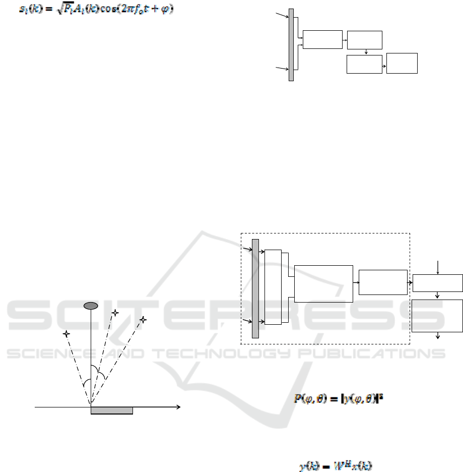
4 SIGNAL PROCESSING
Many sensors for fire detection or building
surveillance are equipped with sound alarm devices.
In case of alarm event (smoke, flame, intrusion,
glass breaking, and unauthorized car opening) the
alarm device generates powerful sound signal with
certain parameters and duration. For the sake of
simplicity, let’s assume that a set of sensors and one
microphone array are installed for the object
protection in the observation area and a video
camera is located above a microphone array as
shown in Fig.3.
Other sound
source Sensor B
Sensor C
Sensor A R
B
R
C
R
A
α
B
α
A
α
C
Microphone array (video camera)
Figure 3: The security system topology
In a security system, the sound source localization
could be used for pointing the additional video
surveillance devices (video cameras) in the needed
directions, which record the additional information
and send it to control center of a security system.
The priority direction for pointing of a video camera
is determined by analysis and identification of
signals received from the detected sound sources.
The analyzed signal parameters used for signal
identification are duration, frequency, modulation,
type (continuous, intermittent), and power. The
general block-scheme of a possible signal processing
in a security system is shown in Fig.4.
x
1
.
.
.
x
M
DOA
Estimation
Parameter
Estimation
Priority
Analysis
Camera
Control
Figure 4: Signal processing in a security system
We assume that the direction of-arrival (DOA) of
sound signals is referred to a Cartesian coordinate
system, the origin of which coincides with the first
element of a microphone array. In a security system,
in which each sensor is equipped with a sound
generator, a microphone array scans the protected
area of observation in an electronic way (Fig.5). In
the process of scanning, a microphone array with a
predetermined angular step directs its main beam in
a certain direction.
x
1
H
. . .
. . .
. . .
x
M
2D-Beam pattern calculation
H
I
L
B
E
R
T
Adaptive
Beamforming
(MVDR)
Power
Estimation
Angular
Coordinates
Estimation
Detection
Figure 5: The block-scheme of DOA estimation
At the output of a microphone array, the signal
power received from any direction is estimated as:
(13)
In (13), y and P are the output signal and the output
power of a microphone array steered in the (β,θ)-
direction (β - azimuth and θ - elevation). The output
of a microphone array with M elements is formed as:
(14)
where k is the time instant, and x(k) is the complex
vector of array observations, W=[w
1
,w
2
,…w
M
]
T
is the
complex vector of the beamformer weights, T and H
denote transpose and conjugate transpose,
respectively. The conventional (delay-and-sum)
beamformer is the simplest, with all its weights of
equal magnitudes and the phases that are selected to
steer the array in particular direction, i.e. the
complex vector of weights W is equal to the array
response vector a
c
, which is defined by the array
configuration. The conventional non-adaptive
beamformer has unity response in each look
direction, that is, the mean output power of the
beamformer in the look direction is the same as the
Second International Conference on Telecommunications and Remote Sensing
88

received source power. In conditions of no
directional interferences, this beamformer provides
maximum SNR but it is not effective in the presence
of the other directional signals, intentional or
unintentional. The others beamformers such as a
Minimum Variance Distortionless Response
beamformer can overcome this problem by
suppressing unwanted signals from off-axis
directions (Tummonery, 1994; Vouras, 2008). To
suppress unwanted signals, this beamformer does
not require the a priori information about them. It
requires only the information for the direction-of-
arrival of expected signals. In this paper we propose
to form the signal y according to the adaptive
MVDR method. The MVDR-beamformer adaptively
calculates the vector of weights (W) providing the
maximum gain in the desired direction while
minimizing the power in the other directions.
According to this method, the optimal weight vector
(W) is chosen to maximize the signal to interference
plus noise ratio (SINR) in a certain direction
:
(15)
In (15), K is the “interference + noise”
covariance matrix of size (M x M), σS2 is the signal
power, and ac is the array response vector in the (,
θ) direction determined by an array configuration.
The solution is found by linear constrained
optimization. The criterion of optimization is
formulated as:
(1)
The solution of (16) gives the following weights:
Many practical applications of MVDR-
beamformers require online calculation of the
weights according to (17), and it means that the
covariance matrix K should be estimated and
inverted online. However, this operation is very
computationally expensive and it may be difficult to
estimate the sample covariance matrix in real time if
the number of samples is large. Furthermore, the
numerical calculation of the weights WMVDR using
the expression (17) may be very unstable if the
sample covariance matrix is ill-conditioned. A
numerical stable and computationally efficient
algorithm can be obtained by using QR
decomposition of the incoming signal matrix. This
matrix is decomposed as X=QR, where Q is the
unitary matrix and R is the upper triangular matrix.
Hence the QR-based algorithm for calculation of
beamformer weights includes the following three
stages:
The linear equation system
c
H
azR =
1
is solved
for
1
z
, and the solution is
c
H
aRz
1*
1
)(
−
=
The linear equation system
*
12
zRz =
is solved
for
2
z
, and the solution is
*
1
1*
2
zRz
−
=
The weight vector
W
is obtained as
)/(
*
2
*
2
zazW
H
c
=
In the process of scanning of the observation
area, the microphone array is digitally steered in
each angular direction (,θ). After adaptive
beamforming of a microphone array in the direction
(,θ), the signal power at the output of a
microphone array is stored, forming in this way the
beam pattern of a microphone array i.e. P(φ,θ). Next,
firstly the local maximums of the obtained beam
pattern must be found and after that they are
compared with a fixed predetermined threshold H. If
some local maximum of the beam pattern, i.e.
Pmax,i(φ*,θ*), corresponding to some angular
direction (φ *,θ*) exceeds the threshold H, then this
angular direction (φ *,θ*) is the estimate of the
DOA.
5 PARALLEL ALGORITHM
5.1 Algorithm Description
Parallel version of the algorithm for DOA estimation
is implemented as a program in Blue Gene
environment using the interface MPI. The parallel
program calculates the signal power at the output of
a microphone array simultaneously for all directions
of observation (Fig.5). The structure of the parallel
program uses the fact that the server loads one the
same copy of the program on all processors from 0
to (NumProc - 1) where NumProc is the number of
processors allocated to the program. The program
uses the current processor number iD, which is
defined by MPI-subroutine MPI_COMM_RANK, in
order to determine which of the two processes to be
performed (depending on that whether the processor
is a master processor, i.e. iD = 0 or slave processor,
i.e. iD> 0). The master processor (iD = 0) performs
initialization of parameters and prepares the data for
all processors. This processor performs simulation
Sound Source Localization in a Security System Using a Microphone Array
89

of signals (or, in practice, reading the signals from
the buffer), in result of which the signal matrix X is
formed. Moreover, for each slave processor, the
main processor calculates the angular direction
(FFI), for which the slave processor (iD = 1 ...
NumProc -1) calculates the signal power at the
output of an adaptive microphone array. The angular
direction (FFI), in which the microphone array is
steered, is sent from the master processor to each
slave processor using the loop organized by the
MPI-subroutine MPI_Send. The main processor also
prepares its data portion (FFI = -90 º and an array
FFI (i), i = 1 ... NumProc, which contains all angular
directions). Then all processors perform identical
calculations - each of them determines the signal
power at the output of a microphone array for
angular direction FFI, using the subroutine
DIAG_AZ_PAR. Once calculating the signal power
at the output of a microphone array, each slave
processor sends the resulting value to the master
processor via the MPI-subroutine MPI_Send.
The master processor via the MPI-function
MPI_Recv accepts the results from all slave
processors and forms the beam pattern of the
microphone array. After that the subroutine
FIND_AZIMUTH finds the angular positions of all
local maximums of the beam pattern, which exceed
the predetermined threshold H. The angular
positions of local maximums are the directions of
arrival of sound of signals. The number of
processors NumProc is equal to the number of
(,θ)- directions used in calculation of the beam
pattern of a
microphone array. At step 2º, the
number of processors is equal to NumProc = (180º
/2º +1) = 91.
5.2 Create and Run the Executable File
Firstly, in Blue Gene environment with the interface
MPI, the executable file, for example,
SOUND_F_PAR.exe, is created using the pre-
created file makesound_F_PAR.txt, which is started
with the command make:
> make-f makesound_F_PAR.txt
With this command all program modules of the
program package are translated and, as a result, the
executable file SOUND_F_PAR.exe is created. The
executable file SOUND_F_PAR.exe is run using
the control file SOUND_F_PAR.jcf (Job Control
File) with the following command:
> llsubmit SOUND_F_PAR.jcf
After the execution the system responds with a
message like:
llsubmit:
Figure 6: Parallel version of the algorithm
i
D=0
?
Y
es
–
Master
C
ALL MPI
_
BCAST of
Х
DO i=1, 2, …… NumProc-1
Calculation of FFI
MPI_Send of FFI
Form the data for the initial
direction
Receive FFI
Calculate the signal power P using
Х
and FFI
CALL DIAG_AZ_PAR(…)
Receive the results
from each and every
one processor:
DO i=1…
N
umProc
-
1
Combine all results:
CALL FIND_AZIMUTH
()
Send the result
to the Master
processor
:
CALL
MPI
S
end
C
ALL MPI
_
Finalize(ierr)
No – Slave
i
D=0
Y
es
–
Master
No – Slave
Initialization of MPI variables:
C
ALL MPI_INIT(ierr);
CALL
M
PI_COMM_SIZE(MPI_COMM_WORLD,
N
umProc,ierr);
CALL
M
PI COMM RANK
(
MPI COMM WORLD
,
Second International Conference on Telecommunications and Remote Sensing
90

The job "bgpfen.daits.government.bg. < task
number>" has been submitted.
The content of the control file
SOUND_F_PAR.jcf can be like that:
# @ job_name = SoundDetect
# @ comment = "SoundDetect :BlueGene"
# @ error = $(jobid).err
# @ output = $(jobid).out
# @ environment = COPY_ALL;
# @ wall_clock_limit = 01:00:00
# @ notification = error
# @ notify_user = never
# @ job_type = bluegene
# @ bg_size = 128
# @ class = n0128
# @ queue
/bgsys/drivers/ppcfloor/bin/mpirun
-exe SOUND_F_PAR.exe -verbose 1
-mode VN -np 91
The number of processors np in the file
SOUND_F_PAR.jcf given above, equals to the
number of angular (for example, azimuthal)
directions, which were used in the formation of the
beam pattern of a microphone array. At step 2º, the
number of processors is equal to np = 91
.
6 SIMULATION RESULTS
The computer simulation is performed to verify the
described algorithm for sound source localization.
As shown in Fig.3, the scenario of simulation
includes three sensors (A, B and C) located
respectively at 50m, 60m and 70m away from the
microphone array. In order to evaluate the
performance of the algorithm for DOA estimation
when using different types of sensors, the
parameters of the sensors produced by three well-
known companies (SONITRON, E2S and SYSTEM
SENSOR) are used in simulation.
Depending of the company of production, the
sirens of sensors generate sound signals at frequency
f0 with the power LW in range from 96dB to 103 dB
(Table 1). In simulation we assume that all sensors
in the protected area are produced by the same
company
.
According to the simulation scenario, the source
of natural noise is a car located in the perpendicular
direction relative to the microphone array.
The horn of this car generates a sound, whose
power is 110dB (Fig.3). The distance to the car is
90m.
Table 1: Sensor parameters
Company
Signal
power
LW [dB]
Sound
frequency
[Hz]
SONITRON 96 2500
E2S 100 1000
SYSTEM
SENSOR
103 2400
Figure 7: Microphone array WA 0807
Two microphone array configurations, the
uniform linear array (ULA) and the uniform
rectangular array (URA), are simulated for each
sensor type. The topology of a microphone array
WA 0807 of the company Brüel & Kjær is used in
simulation (Fig.7).
• The Brüel&Kjær microphone array
parameters are:
• Frequency, at which the controlled sensors
generate the sound (Hz);
• Array configuration (linear, rectangular,
square);
• Distance between array microphones (d),
which can be changed for each type of
sensors;
• Total number of microphones in the
microphone array.
The parameters of microphones of the type 4935
according to the catalogue of the company Brüel &
Kjær are used in simulation of the microphone array
(Fig.8).
Figure 8: Microphone 4935 (Brüel & Kjær)
Sound Source Localization in a Security System Using a Microphone Array
91

The noise level of such a microphone is 35dB in
the frequency range [100 - 5000] Hz. It is assumed
that all simulated microphone arrays (ULA and
URA) have the same overall dimension of 0.5m. The
interelement spacing of each microphone array and
as a consequence the corresponding number of
elements are determined according to the carrier
frequency of a signal generated by the sound source.
For each type of sensors, the interelement
distance in a microphone array is calculated as d = λ
/ 2, where λ is the wavelength of the sound
generated by a sensor. The sound wavelength
depends on the frequency of the generated sound,
i.e. λ = c/f0, where c = 344 m/s is the propagation
velocity of sound in air, and f0 is the frequency of
the acoustic signal (Table 1). The signal amplitude
(A) at the output of each microphone of a
microphone array is calculated as a function of the
sound pressure LP:
(18)
In (18), the sound pressure LP (in dB) depends
on the power of the sound LW, which is different for
each sensor (Table 1) and also depends on the
distance R to the sound source:
(19)
The real and estimated values of the DOA are
presented in Table 2 for each type of a microphone
array. The beam patterns of the microphone arrays
are presented respectively in Fig.9 … Fig.14.
Table 2: True and estimated azimuthal directions
SENSOR
TYPE
Array
Type
Source
Azimuth
[°]
Estimated
Azimuth [°]
ULA
(11x1)
-14;0;14;28 -14; 0;14; 28 SONITRON
URA
(11x4)
-14;0;14;28 -14; 0; 14; 28
ULA
(4x1)
-26; 0; 26 -26; 0; 26 E2S
URA
(4x4)
-26;0;26;52 -26; 0; 26; 52
ULA
(8x1)
-14;0;14;28 -14; 0;14; 28 SYSTEM
SENSOR
URA
(8x4)
-14;0;14;28 -14; 0;14; 28
The number of directions, for example, in
azimuth (NAZ), controlled by a microphone array
depends on the angular resolution of the microphone
array (Δ), which in its turn is determined by the
geometrical configuration of the microphone array
and the number of its elements:
(20)
The angular resolution Δφ is determined as the
width of the main lobe of the beam pattern created
by a microphone array. Comparing the plotted beam
pattern presented on Fig.9…Fig.14, it can be seen
that the best angular resolution in azimuth is
provided by using the microphone array ULA-11
(with 11 microphones) and opposite, the worst
angular resolution is provided by using the
microphone array ULA-4 (with 4 microphones).
Therefore, the ability of a microphone array to
separate
the signals from different sound
sources is improved with increasing the
number of microphones in the array.
Figure 9: Beam pattern of the URA-8x4 (Sensor
Type –SYSTEM SENSOR)
Figure 10: Beam pattern of the ULA-8x4 (Sensor Type –
SYSTEM SENSOR)
Second International Conference on Telecommunications and Remote Sensing
92
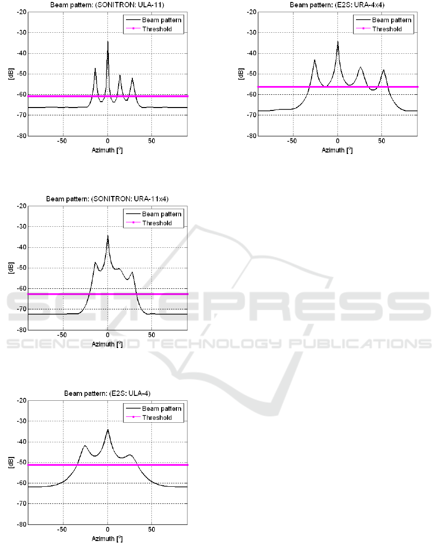
Figure 11: Beam pattern of the ULA-11 (Sensor
Type –SONITRON)
Figure 12: Beam pattern of the URA-11x4 (Sensor
Type –SONITRON)
Figure 13: Beam pattern of the ULA- 4x1 (Sensor
Type –E2S)
Figure 14: Beam pattern of the URA- 4x4 (Sensor
Type –E2S)
It is well known that the maximal number of signals
arrived from different directions, which can be
separated by a microphone array, equals (M-1),
where M is the number of array elements.
Therefore, the beam pattern plotted in Fig. 13 shows
that the microphone array ULA-4 can separate only
3 sound signals received from different directions
and generated by 3 E2S sensors. The graphical
results also show that linear microphone arrays
(ULA) should be used in cases where it is important
to control the movement of the video camera only in
azimuthal direction. However, when it is important
to control the movement of the video camera in 2D
space (azimuth and elevation), you must use
rectangular microphone arrays (URA). Comparison
analysis of the beam patterns plotted in Fig. 11 (for
ULA-11, SONITRON) and Fig.12 (for URA-11x4,
SONITRON) shows, that the use of a rectangular
microphone reduces the angular resolution in
azimuth
.
7 CONCLUSIONS
The results obtained show that the accurate
DOA estimates can be obtained using a
microphone array if the adaptive MVDR-
algorithm is used for beamforming. It is
also shown that the maximal number of
separated signals and also the effectiveness
of microphone arrays depend on the number
of array elements. Finally, the results
obtained can be successfully used for solving
different problems associated with noise source
localization and identification.
Sound Source Localization in a Security System Using a Microphone Array
93

ACKNOWLEDGEMENTS
The research work reported in the paper is partly
supported by the project AComIn "Advanced
Computing for Innovation", grant 316087, funded by
the FP7 Capacity Programme (Research Potential of
Convergence Regions).
REFERENCES
Benesty, J., Chen, J., Huang, Y., 2008. Microphone array
signal processing, Springer.
Godara, L., 1997. Application of antenna arrays to mobile
communications, part II: beam-forming and direction-
of-arrival considerations. In Proc. of the IEEE, vol.85,
No 8, pp.1195-1245.
Ioannides, P., Balanis, C., 2005. Uniform circular and
rectangular arrays for adaptive beamforming
applications. IEEE Trans. on Antenna. Wireless
Propagation. Letters, vol.4., pp. 351-354.
Trees, H., Van, L., 2002. Optimum Array Processing. Part
IV. Detection, Estimation, and Modulation Theory.
New York, JohnWiley and Sons, Inc..
Tummonery, L., Proudler, I., Farina, A., McWhirter, J.,
1994. QRD-based MVDR algorithm for adaptive
multi-pulse antenna array signal processing. In Proc.
Radar, Sonar, Navigation, vol.141, No 2, pp. 93-102.
Vouras, P., Freburger, B., 2008. Application of adaptive
beamforming techniques to HF radar. In Proc. IEEE
conf. RADAR’08, May, pp. 6.
Moelker, D.,VandePol, E., 1996. Adaptive Antenna Arrays
for Interference Cancellation in GPS and GLONASS
Receivers. In Proc. of the IEEE symp. on Position
Location and Navigation, April, pp.191-196.
http://sonitron.be/site/index.php,\
http://www.e2s.com/
http://www.systemsensor.com/
Second International Conference on Telecommunications and Remote Sensing
94
