
VALIDATION OF TWO NEW EMPIRICAL IONOSPHERIC
MODELS IRI-PLAS AND NGM DESCRIBING CONDITIONS OF
RADIO WAVE PROPAGATION IN SPACE
Maltseva Olga, Mozhaeva Natalia, Vinnik Elena
Institute of Physics Southern Federal University, Stachki, 194, Rostov-on-Don, Russia
mal@ip.rsu.ru, mozh_75@mail.ru
Keywords: GPS. Total electron content. Ionospheric model. Radio wave propagation. Geomagnetic disturbances.
CHAMP. DMSP
Abstract: An empirical modeling of the behavior of ionospheric parameters is an important goal. The most
complicated it is for the total electron content (TEC). The article focuses on two approaches: 1) the
integration of N(h)-profiles using empirical parameters foF2 and hmF2, 2) the use of experimental values of
the TEC. In recent years, two new models were developed: 1) IRI-Plas as a representative of the first
approach, and 2) the Neustrelitz Global Model (NGM) as a representative of the second approach. Both
models have their advantages over previous models. Any new model needs to be tested to get a quantitative
estimate of proximity between the model and experiment, but both models have not been tested yet by
anyone other than the authors of models. This article is dedicated to such testing. Besides the traditional
comparison of model parameters foF2 and TEC with experimental data, in the paper the testing of additional
parameters was performed with the help of independent experiments. For the IRI-Plas model, these are
N(h)-profiles, data of incoherent scatter radars, and plasma frequency, measured at a height of satellites. For
the NGM model, this is the equivalent slab thickness of the ionosphere τ. For the European region, it is
shown that in most cases, the IRI-Plas model may be preferred to determine the parameters foF2 and TEC.
For the parameter τ(NGM), there are conditions under which τ(NGM) provides better results than τ(IRI).
1 INTRODUCTION
Ionospheric models play an important role in
determining wave propagation conditions of
different frequency ranges in the nearest Earth
space. The main parameters are the critical
frequency foF2, the maximum height hmF2, the total
electron content TEC. The most important parameter
to operate navigation and communication systems is
the TEC (e.g. Goodman, 2005). Positioning
accuracy is directly proportional to the TEC. It can
also be used to determine foF2 (Maltseva et al.,
2012a). The article focuses on two approaches: 1)
the integration of N(h)-profiles using empirical
parameters foF2 and hmF2, 2) the use of
experimental values of the TEC. The disadvantage
of the first approach is the large discrepancy
between model and experimental values of the TEC
(Maltseva, Zhbankov, Nikitenko, 2011). In the
second approach, there was no global empirical
model of the TEC, and the existing regional models
provide a large range of values TEC (up to an order
of magnitude) (e.g. Arican, Erol, Arican, 2003). In
recent years, two new models were developed: 1) the
IRI-Plas model (Gulyaeva, 2011) and 2) the
Neustrelitz Global Model (Jakowski, Hoque, Mayer,
2011). In this paper, it is abbreviated by NGM. The
IRI-Plas model refers to the first approach, the NGM
model - to the second one. Both models have their
advantages. The IRI-Plas model introduces the
topside basis scale height Hsc, which improves the
shape of the N(h)-profile, and takes into account a
plasmaspheric part of the profile. As for the NGM
model, according to (Jakowski et al., 2011) this
empirical model can be operated autonomously
without any ionospheric measurements. To
characterize the solar activity dependency, the 10.7-
cm flux of the Sun is used as a proxy for the ionizing
extreme ultraviolet radiation. The model is easy to
handle and can efficiently be used in single
frequency GNSS and radar systems for estimating
109
Olga M., Natalia M. and Elena V.
VALIDATION OF TWO NEW EMPIRICAL IONOSPHERIC MODELS IRI-PLAS AND NGM DESCRIBING CONDITIONS OF RADIO WAVE PROPAGATION IN SPACE.
DOI: 10.5220/0004786001090118
In Proceedings of the Second International Conference on Telecommunications and Remote Sensing (ICTRS 2013), pages 109-118
ISBN: 978-989-8565-57-0
Copyright
c
2013 by SCITEPRESS – Science and Technology Publications, Lda. All rights reserved

range error or ionosphere related polarization
changes by the Faraday effect. (p. 966).
Both models need to be tested, since no one
other, than the authors themselves, did test these
models. In this paper, testing will be conducted as to
the common parameters (foF2 and TEC), allowing
us to compare
the results of both models to each
other, and to the parameters that the authors did not
test, but which are of great practical importance. In
the first case, these are N(h)-profiles. They are tested
by data of incoherent scatter radars and plasma
frequency, measured at a height of satellites. In the
second case, the model allows to determine the
equivalent slab
thickness of the ionosphere τ(NGM)
= TEC(NGM) / NmF2(NGM). This parameter also
needs an empirical model
but doesn’t have it. The
relevant test is to
show whether can τ(NGM) be an
empirical model of the equivalent slab thickness of
the ionosphere.
2 DATA AND MODELS USED
Experimental data of TEC values are used from the
global maps of JPL, CODE, UPC, ESA, which are
calculated from IONEX files (ftp://cddis.gsfc.nasa.
gov/pub/gps/products/ionex/) for given coordinates
and time points. Values of other parameters of the
ionosphere were taken from the SPIDR database
(http://spidr.ngdc.nasa.gov/ spidr/index.jsp). Of the
model, as indicated in the Introduction, there are two
ones: IRI-Plas and NGM. The IRI model is well
known and widely used. It is presented in some
detail in the work (Maltseva, Mozhaeva, Zhbankov,
2012, below paper1) and in many others. Since the
NGM model is completely new, it is necessary to
give its brief description. A global model of the
TEC(NGM) is given by product of five multipliers:
TEC(NGM) = F1 * F2 * F3 * F4 * F5.
It is based on data of the global CODE map. Each
multiplier reflects the dependence of TEC on certain
physical factors and is calculated using 2 to 6
coefficients CI. Coefficients are determined by the
least-squares procedure superimposed on
experimental data for several years. Coefficient F1
describes the dependence of TEC on the local time
LT, i.e. on a solar zenith angle, and includes daily,
half-day, 8-hour variations. It is calculated using 5
coefficients (C1-C5). Maximum of daily variations
is shifted to LT = 14. Coefficient F2 describes
annual and semi-annual variations, using
coefficients C6-C7. Coefficient C8 is included in the
F3 multiplier describing the dependence of the TEC
on the geomagnetic latitude. Coefficients C9 and
C10 correspond to accounting equatorial anomalies
in the latitude dependence of the TEC (factor F4).
Coefficients C11 and C12 describe the dependence
of the TEC on the index F10.7: F5=
C11+C12*F10.7. A model for NmF2 (Hoque and
Jakowski, 2011) is built on the same principle, but
has 13 coefficients, since in this case the factor F1 of
daily course includes 6 coefficients. Maximum of
daily variation is also shifted to LT = 14. A model of
hmF2 (Hoque and Jakowski, 2012) includes 4
multipliers: hmF2=F1*F2*F3*F4, because there is
no special factor of the equatorial anomaly. F10.7
values are tied to the number of days of a year.
Dependence on F10.7 is described by the factor F4.
Below we give a comparison of parameters of the
two models with experimental data and with each
other. Results are represented using data of the
Juliusruh station (in the main), located in the central
part of Europe.
3 TESTING MODELS BY IS
RADARS
As noted, because a value of TEC of the IRI
model is calculated by integrating N(h)-profiles, it is
important to test the profile shape with the help of
independent experiments. One of them is incoherent
scatter radars (ISR). Paper1 (Section 3) represented
results of testing IRI-Plas according to three radars
on the borders of the European zone near the
maximum of solar activity. In recent years, much
attention was paid to peculiarities of simulation
results of ionospheric parameters and N(h)-profiles
during periods of low activity (Cander and
Haralambous, 2011; Liu et al., 2011; Zakharenkova
et al., 2013; Cherniak et al., 2012; Maltseva,
Mozhaeva, Nikitenko, Thinh Quang, 2012). This is
all the more relevant as the forecast of maximum of
the 24 cycle will be less than the maximum of the 23
cycle, and the 25 cycle will be even less powerful, as
can be seen from Fig. 1 (from http://
solarscience.msfc.nasa.gov/predict.shtml).
Data of the Kharkov radar (49.6°N, 39.6°E),
located in the central part of Europe, allow to fulfill
an additional test for the conditions of the minimum
activity.
According to data for two years (2007-2008), the
authors (Cherniak,Zakharenkova, Dzyubanov, 2013)
were able to select only the two days: 25 September
2007 and 29 October 2008. Both days are
Second International Conference on Telecommunications and Remote Sensing
110
characterized by quiet geomagnetic conditions.
Authors (Cherniak et al., 2013) compared critical
frequencies foF2 of ISR with results of the Juliusruh
station (54.6°N, 13.38°E).
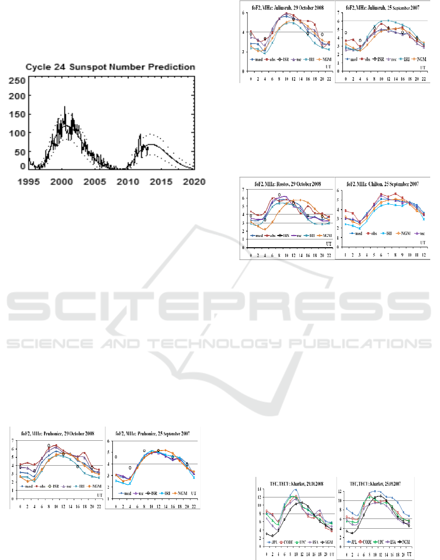
Figure 1. Solar number prediction for the 24 cycle
We compared them with results of the Průhonice
station (50°N, 14.5°E), which is closer to the
Kharkov radar than the Juliusruh station. Fig. 2
shows the daily run of foF2 for the following cases:
1) monthly median of foF2 (icon “med”), 2) the
experimental value (“obs)”, 3) data of ISR, 4) values
of foF2(rec), calculated using τ(med) of the JPL map
(Paper1), 5) the value of the original IRI model,
which is the median, 6) the value of the NGM
model. Unlike the IRI model, which uses moving
12-month indices RZ12, the NGM model formally
defines not only the median (they just still need to be
calculated from the values for the daily F10.7), but
also the value for a particular day. The left panel
refers to 29/10/2008, right – to 25/09/2007. In Fig. 3,
these dependences are shown for the Juliusruh
station.
Figure 2. Comparison of various options of the foF2
determination (selected days, the Pruhonice station)
In Fig. 3, these dependences are shown for the
Juliusruh station.
Figure 3. Comparison of various options of the foF2
determination (selected days, the Juliusruh station)
For completeness, the results are given for the
Rostov station closest to the radar (data of this
station were not available for October 2007), and
Chilton at 09/25/2007 (fig. 4).
Figure 4. Comparison of various options of the foF2
determination (two stations)
Even these few graphs allow us to make some
conclusions: with two exceptions of September 25,
2007 (2UT and 4UT), values for both models are
fairly well with the experiment as medians and foF2
values on specific days. Quantitative deviations
|ΔfoF2| are minimal for foF2(rec) and maximum for
foF2(IRI) or foF2(NGM). It is difficult to give
preference to one of the models. For all 12 cases of
ISR data, N(h)-profiles were calculated for the
original model, and for adaptation of the model to
the experimental values of various parameters,
separately for cases of foF2, TEC and their joint use.
Unlike paper1, an additional adjustment to the
TEC(NGM) was added. The whole set of values of
the TEC is shown in Fig. 5.
Figure 5. Comparison of various options of the TEC
determination for the two days of Kharkov ISR
measurements
Validation of Two New Empirical Ionospheric Models IRI-Plas and NGM Describing Conditions ....
111
Examples comparing N(h)-profiles with ISR profiles
for the various options are shown in Fig. 6 for night
(0 UT) and day (16 UT) conditions. This comparison
has several objectives: a) to determine the map the
N(h)-profile of which is the closest to the ISR
profile, b) to determine the N(h)-profile for
TEC(NGM).
Figure 6. Comparison of N(h)-profiles calculated with
N(h)-profiles of the Kharkov ISR
Figure 7. Comparison of model results with ones of global
maps
It can be seen that the correspondence of N(h)-
profiles are very different in day and night
conditions. Daily profiles for all TEC options
including TEC(NGM) are very close to the ISR
profile. At night, only the N(h)-profile of the JPL
map is close to the ISR profile. It is necessary to
note that the JPL map gives the highest values of
TEC. Profile for the NGM model shows virtually no
ionization in the upper ionosphere, it is hard to
imagine even in period of the minimum activity. A
more complete picture is given by the analysis of all
12 cases. Fig. 7 (the left panel) shows the absolute
deviations of the plasma frequency fne(600) and
their dispersion (in MHz). They were obtained as the
average for all days. The right panel displays the
dispersion in %. This dispersion is important when
comparing the results for different conditions of
solar activity, because the relative dispersion is less
dependent on RZ12, than absolute. The values are
sorted from maximum to minimum to highlight an
option with the maximum and minimum deviation.
We see that in this case, the maximum deviations
correspond to the NGM model, minimum – to the
JPL map. Fig. 8 shows the values of fne(h = 600) for
the profiles of ISR, NGM and JPL (the left panel).
The right side shows their deviation. The abscissa is
date of the measurement for the two selected days.
Figure 8. Comparison of plasma frequencies and their
deviations for the two selected days and the two models
4 COMPARING THE
CONFORMITY OF
IONOSPHERIC PARAMETERS
Fig. 6 of the previous Section shows that the
deviation of the JPL map does not exceed a certain
value, and the NGM model is characterized by large
deviations at night. This Section provides an
illustration of conformity of ionospheric parameters
of the two models to the experimental data for the
conditions of varying solar activity..
Figure 9. Examples of appropriate foF2 for different levels
of solar activity (May, various years)
Comparison was made for medians of the
corresponding parameters. Fig. 9 shows a
comparison of foF2(med) for May. Fig. 10
represents results for December
Second International Conference on Telecommunications and Remote Sensing
112
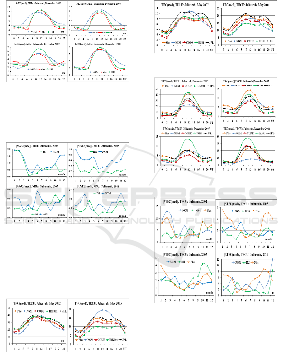
Figure 10. Examples of appropriate foF2 for different
levels of solar activity (December, various years)
It is seen that in May and December the NGM
model does not reflect the characteristics of diurnal
values of foF2 (med). Examples of seasonal
differences are shown in Fig. 11.
Figure 11. Examples of seasonal conformity foF2 for
different levels of solar activity
Figures 12-14 represent similar results for the
TEC. Here are experimental values of TEC(CODE).
Additionally results of the JPL map are given,
because its values are most commonly used in
applications. For the IRI model, results are reported
for 2 versions: IRI-Plas and IRI2001 (Bilitza, 2001).
Figure 12. Examples of relevant TEC for different levels
of solar activity (May, various years)
Figure 13. Examples of relevant TEC for different levels
of solar activity (December, various years)
Figure 14. Examples of seasonal conformity of TEC for
different levels of solar activity
As can be seen from Fig. 14, the value of this
particular version is closest to the experimental
TEC.
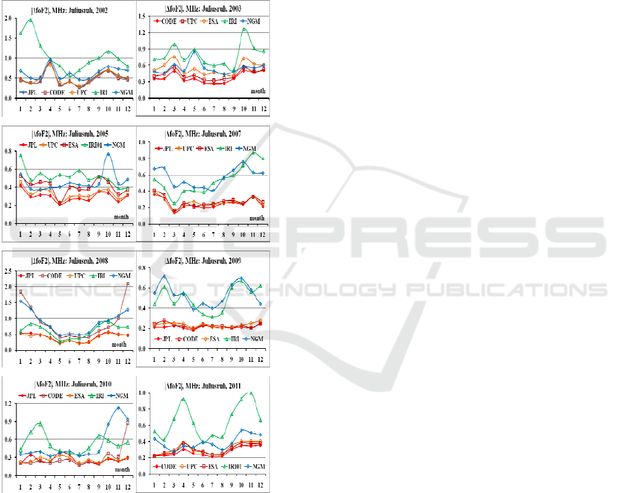
As for the two models, the IRI-Plas model often
overestimates the value of TEC (compared with
CODE), and hence gives greater deviations than
NGM. Relative deviations in % are given in Table 1.
Validation of Two New Empirical Ionospheric Models IRI-Plas and NGM Describing Conditions ....
113
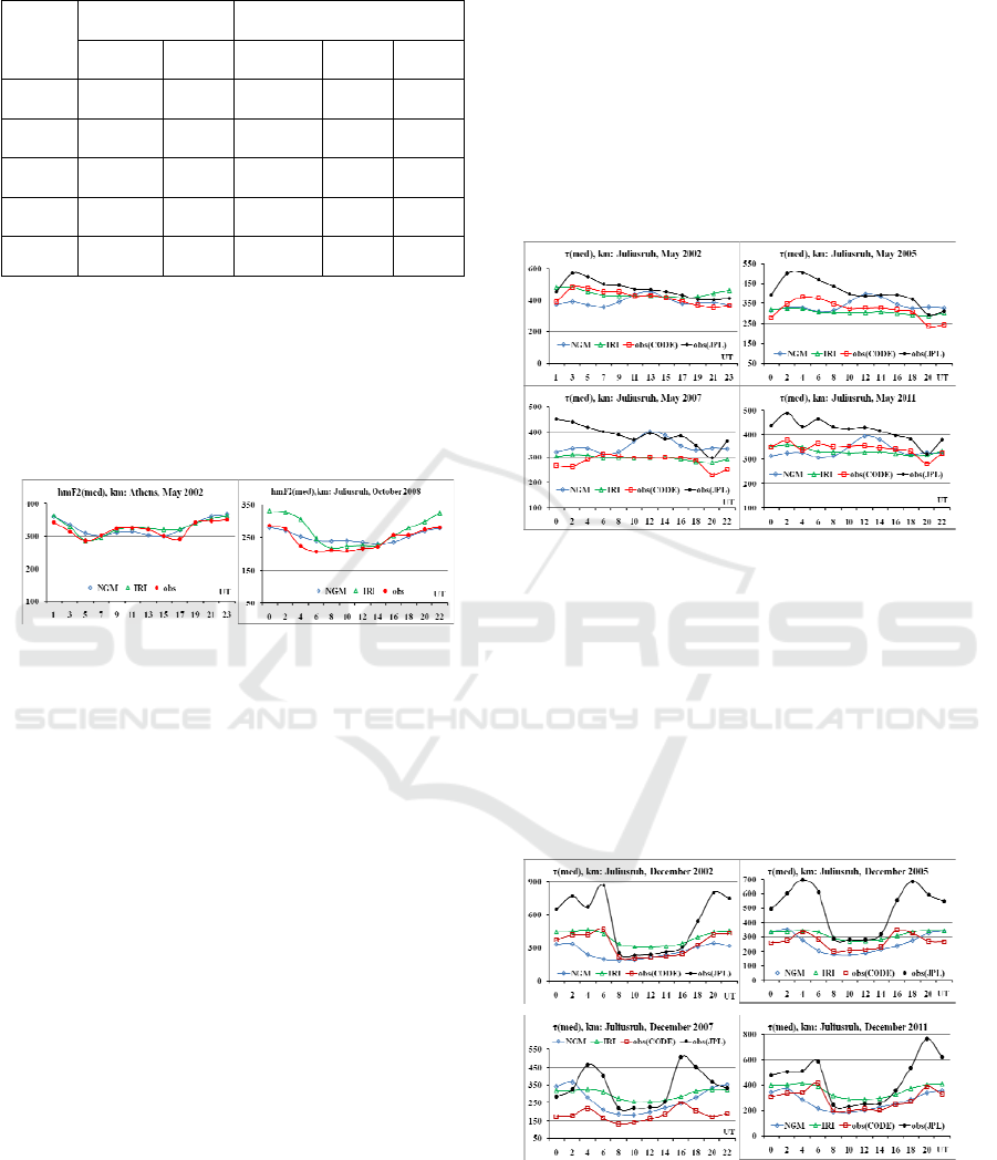
Table 1. Comparison of relative deviations for the two
parameters of the ionosphere for the Juliusruh station
у(foF2),% у(TEC),%
NGM IRI NGM IRI Plas
2002 18.3 11.8 30.8 25.5 29.1
2005 17.7 6.5 34.3 29.7 56.0
2007 15.3 12.0 44.8 69.2 51.2
2008 19.0 20.0 96.3 57.0 125.
2011 18.1 10.3 40.7 27.8 62.7
As for the parameter hmF2, then it is more
difficult to make the test for it, because experimental
data are very limited. Fig. 15 shows the curves for
maximum activity (May 2002, the Athens station)
and for minimum (October 2008, the Juliusruh
station).
Figure 15. Examples of compliance of hmF2
On the one hand, there is a tendency inherent in
the first two parameters: the deviation is less for
both models in near maximum solar conditions, on
the other hand, in both cases, the NGM model
provides results that are 2 times better than the IRI
(relative deviations are 5 and 10% in the first case
and 8 and 15% in the second one.)
5 COMPARISON OF RESULTS
FOR THE MEDIAN OF THE
EQUIVALENT SLAB
THICKNESS OF THE
IONOSPHERE τ(MED)
Parameter τ (= TEC/NmF2) may play a role in
assessing the state of the ionosphere. In (Gulyaeva,
2011), a formula between parameters Hsc (the
topside basis scale height) and foF2 was obtained,
allowing (maybe) to predict the behavior of this
parameter during disturbances. Since there is a
relationship between τ and Hsc (Hsc is a part of τ), it
is possible, apparently, to get a connection for τ. But
in this work, as in the paper1, we focus on assessing
the possibility of determination of foF2 from
experimental TEC with τ(med). Traditional methods
are based on the use of τ(IRI) (McNamara, 1985;
Houminer and Soicher, 1996; Gulyaeva, 2003), i.e.
NmF2(rec) = TEC(obs)/τ(IRI). Frequency foF2(rec)
is proportional to the square root of NmF2(rec).
Naturally, the calculated values NmF2(rec) will be
the closer to the experimental NmF2(obs), the closer
τ(IRI) to τ(obs).
Figure 16. Examples of appropriate τ(med) for different
levels of solar activity (May, various years)
In this section, these values are determined for
the NGM model, to compare the experimental
values (defined from the CODE map) with τ(IRI)
and τ(NGM). Additionally they show τ(JPL), since
in most cases this map gives the best fit to the
experimental data of foF2. The corresponding results
are shown in Fig. 16-17, which are obtained using
curves of Figs 9-10, 12-13.
Figure 17. Examples of appropriate τ(med) for different
levels of solar activity (December, various years)
These large differences between τ(CODE) and
τ(JPL) should not be discouraged, because they are
obtained from different TEC (TEC(CODE) and
Second International Conference on Telecommunications and Remote Sensing
114
TEC(JPL)). Authors (Jakowski et al., 2011) selected
the CODE map. If they chose the JPL map, the
results would have been closer to τ(JPL). As can be
seen from these Figures, almost all the values of
τ(NGM) are closer to the experimental τ(CODE),
than τ(IRI), therefore, foF2(rec) for τ(NGM) should
be closer to the foF2(obs) than foF2(IRI). To
confirm this important fact and assess the possible
use of τ(NGM) for the determination of foF2,
calculations were fulfilled for IRI, NGM, and
different maps (Fig. 18).
Figure 18. The absolute difference between experimental
frequencies foF2 and frequencies calculated using the
values of medians of τ for global maps of JPL, CODE,
UPC, ESA and empirical models IRI and NGM
It turned out that the results depend on the level
of solar activity, so we have provided detailed
graphs for several years to illustrate what the
conditions are most favorable for τ(NGM). Each
graph shows the absolute difference between
experimental values foF2(obs) and values foF2(rec),
recovered using appropriate TEC. The general trend
is to ensure that, in determining foF2(rec) from the
TEC best results are obtained for the JPL map. The
"second" place belongs to the CODE map. As for
NGM, then its deviations |ΔfoF2| are much smaller
than these for the model IRI under the conditions of
high solar activity though they are larger in
magnitude than deviations for global maps. As
already noted, the simulation results in low solar
activity is of great interest because of the evidence
found that the model IRI is worse working in these
conditions (2007-2009) (Zakharenkova et al., 2011;
Maltseva et al., 2012a). Fig. 18 shows that the NGM
model does not improve results compared with the
IRI model. In addition, results for 2008 (the year
with the lowest activity) show that the determination
of the TEC from the CODE map reveals a
significant effect of measurement error on the values
themselves (apparently, the value of error is much
greater than the TEC for this map)
6 TESTING MODELS USING
PLASMA FREQUENCIES
MEASURED BY SATELLITES
Paper1 has attempted to test the IRI model by data
of CHAMP (h ~ 400 km) and DMSP (h ~ 860 km)
satellites. It has been shown that in most cases N(h)-
profiles corresponding to various maps do not
provide an exact match of the plasma frequency
fne(sat) at the height of the satellite, but one can
choose a profile that passes through the foF2(obs)
and plasma frequency of one or two satellites. This
yields a value of TEC, other than the maps. In most
cases, these values fall in the range of maps and
form there an own subset. We use the fne(sat) to
evaluate the situation for the NGM model. The
results are shown in Fig. 19 for stations Juliusruh
and Chilton and the various levels of solar activity.
The red circles show the values of TEC(fne) for
N(h)-profiles passing through fne(sat) of the DMSP
satellite. The remaining values correspond to global
maps (no values of the UPC map, because they are
very close to the values of CODE). Values of TEC
are ordered from maximum to minimum for each
hour of UT, shown on the horizontal axis.
Validation of Two New Empirical Ionospheric Models IRI-Plas and NGM Describing Conditions ....
115
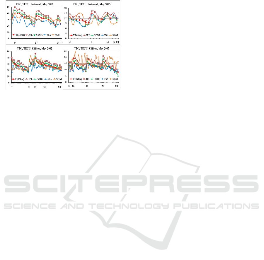
Figure 19. A comparison of different sets of TEC
Fig19 shows: a) the range of possible values for
each of the experimental hour is large, b) TEC is
experiencing great changes for various days and one
hour, but changes are sufficiently synchronized for
all maps. NGM model values, in-first, go far beyond
the experimental range, to-second, within the hour
have large random variation in various days.
7 EXAMPLES OF THE
DISTURBED BEHAVIOR OF
N(h)-PROFILES
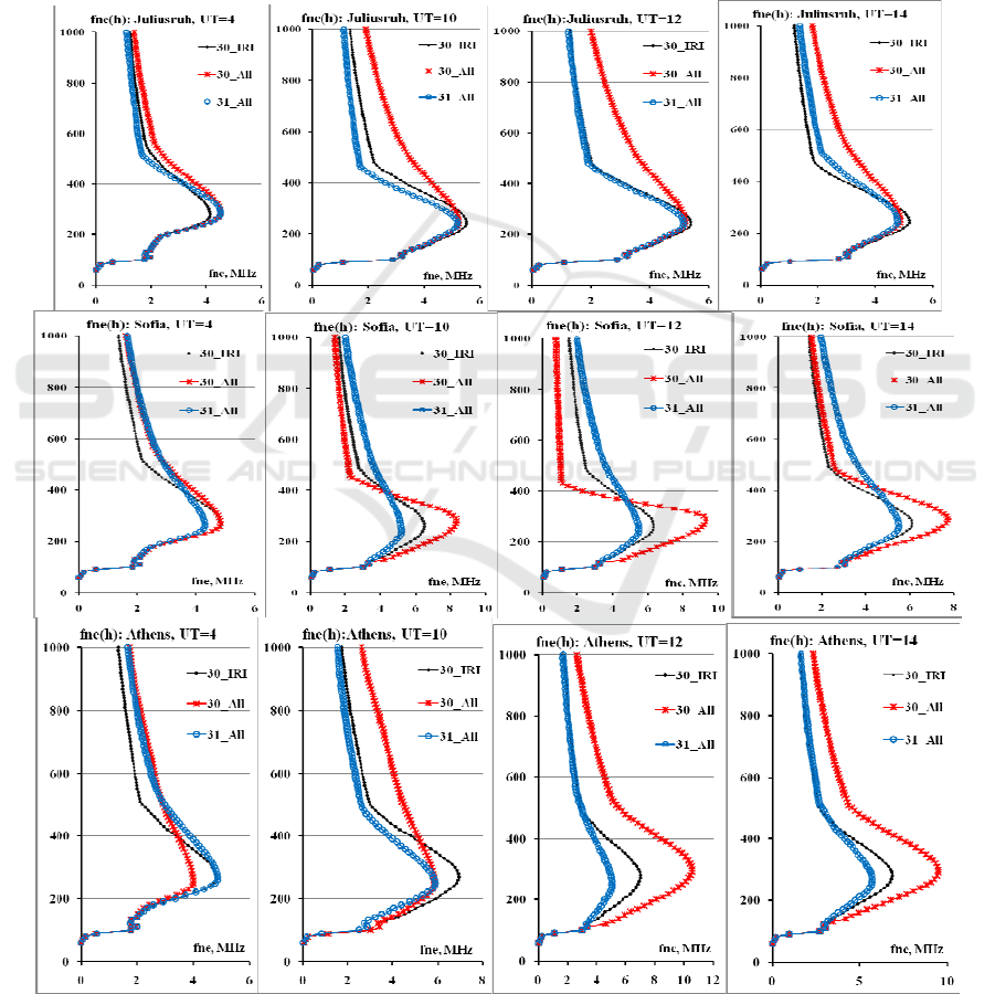
Examples of the disturbed behavior of N(h)-profiles
are represented in Fig. 20 during the last disturbance
of May 2005. The strongest phase of this disturbance
falls on 30 May. One can see response of various
parts of N(h)-profiles on this disturbance in different
latitudes. The top panel concerns to the Juliusruh
station. The middle panel displays results for the
Sofia station. The part of them was given from
paper1 (fig. 10) to compare with new results. The
bottom panel concerns to the Athens station. All
profiles are close to model ones in 4UT (near quiet
conditions). In the next moments 10-14UT, the
positive disturbance over the Juliusruh station is
developed covering only topside profiles. N(h)-
profiles over the Sofia station show redistribution of
ionization, i.e. its increase near hmF2 due to
depletion of the higher part. Conditions over the
Athens station are characterized by input of
ionization from the magnetosphere (10UT), two-fold
increased ionization of the whole profile (12UT).
Phase of recovering (31 May) is faster in the topside
part than in the bottom of the F2 layer, where the
negative disturbance continues during all day. It
shows that N(h)-profiles of the IRI-Plas model can
be used not only in technical applications but to
solve some problems of physics of the ionosphere.
8 CONCLUSION
The paper discusses two new models that
give average values of ionospheric
parameters: the critical frequency foF2, the
maximum height hmF2, the total electron
content TEC. One of them is the IRI-Plas model,
which is a new option of the IRI model, the best
known and most widely used, which is constantly
updated. Its additional testing was held according to
the Kharkov IS radar and the satellite data in a
period of low solar activity. The second one is the
new NGM model (the Neustrelitz Global Model),
which is extremely simple: each parameter is the
product of no more than 5 factors: P =
F1*F2*F3*F4*F5 with clear physical binding of
each factor. Another feature of the model is the
dependence of each parameter on the number of
days in the year and the corresponding index F10.7.
To build the model TEC, its authors selected the
global CODE map. Results obtained confirm the
findings of the paper1 concerning to the high
efficiency of adaptation of the IRI-Plas model to the
experimental values of foF2, hmF2, and TEC.
Further adaptation to the plasma frequency fne,
measured by satellite DMSP, leads to new values of
TEC(fne), which fall in the range of experimental
values of global maps and can be considered as an
independent estimate of the TEC. As regards the
NGM model, for the purposes of its authors, i.e. in
single frequency GNSS and radar systems, it is
possible that the simplicity of the model plays a
crucial role and the model will be used with success.
In principle, the average foF2 and TEC values are
predicted well, and in some cases the NGM model
can give better results than IRI. But for the purposes
of the wave propagation this is not enough, because
the NGM model does not reflect daily variations of
foF2 and TEC, and the discrepancy with the
experimental data and with the IRI model may be
1.5-3 times.
It should be noted that in some cases the best
results for the TEC are provided by the IRI2001
model, whose ceiling of N(h)-profile is 2000 km.
This is due to the fact that the IRI2001 model
strongly overestimates the concentration in the upper
ionosphere (up to 1000 times) and this compensates
for the lack of the plasmaspheric part of the N(h)-
profile. Apparently, the fact that the new IRI-Plas
Second International Conference on Telecommunications and Remote Sensing
116
option also overestimates TEC in some cases,
suggests that the real Hsc of the new profile is
smaller than the model Hsc. As for the median
equivalent thickness of the ionosphere τ(med), then
there are conditions of solar activity, when the NGM
model gives results better than the IRI model. Such a
conclusion cannot be generalized to other regions
without additional testing because of a strong
dependence of the results on the location of the
observation point and the solar activity. We can note
also that previous versions of the IRI model
(IRI2001 (Bilitza, 2001) and IRI2007 (Bilitza and
Reinisch, 2008)) were validating during tens of
years and this validation is continued. Validation of
the IRI-Plas model and the NGM model began just
now.
Figure 20. Development of disturbance of 30-31 May 2005 in N(h)-profiles on different latitudes
Validation of Two New Empirical Ionospheric Models IRI-Plas and NGM Describing Conditions ....
117

ACKNOWLEDGEMENTS
Authors thank organizations and scientists who are
developing the IRI model, providing data of
SPIDR, JPL, CODE, UPC, ESA, Dr M. Hoque for
detailed comments on the NGM model, two
reviewers for useful comments.
REFERENCES
Arikan, F., Erol, C. B., Arikan, O. (2003). Regularized
estimation of vertical total electron content from
Global Positioning System data. Journal of
Geophysical Research, 108(A12), 1469,
doi:10.1029/2002JA009605.
Bilitza, D. (2001). International Reference Ionosphere.
Radio Science, 36(2), 261-275.
Bilitza D., Reinisch, B.W. (2008). International
Reference Ionosphere 2007: Improvements and New
Parameters. Advances in Space Research, 42, 599-
609.
Cander, L.R., Haralambous, H. (2011). On the
importance of TEC enhancements during the
extreme solar minimum. Advances in Space
Research, 47, 304-311.
Cherniak, Iu.V., Zakharenkova, I.E., Dzyubanov, D.A.
(2013a). Accuracy of IRI profiles of ionospheric
density and temperature derived from comparisons
to Kharkov incoherent scatter radar measurements.
Advances in Space Research, 51(4), 639-646.
Cherniak, Iu.V., Zakharenkova, I.E., Krankowski, A.,
Shagimuratov, I.I. (2012b). Plasmaspheric electron
content from GPS TEC and FORMOSAT-3/COSMIC
measurements: solar minimum conditions. Advances
in Space Research, 50(4), 427-440.
Goodman, J.M. (2005). Operational communication
systems and relationships to the ionosphere and
space weather. Advances in Space Research, 36,
2241–2252.
Gulyaeva, T.L. (2003). International standard model of
the Earth’s ionosphere and plasmasphere.
Astronomical and Astrophysical Transaction, 22(4),
639-643.
Gulyaeva, T.L. (2011). Storm time behavior of topside
scale height inferred from the ionosphere-
plasmosphere model driven by the F2 layer peak and
GPS-TEC observations. Advances in Space
Research, 47, 913-920.
Hoque, M.M., Jakowski, N. (2011). A new global
empirical NmF2 model for operational use in radio
systems. Radio Science, 46, RS6015, 1-13.
Hoque, M.M., Jakowski, N. (2012). A new global model
for the ionospheric F2 peak height for radio wave
propagation. Annales Geophysicae, 30, 797-809.
Houminer, Z., Soicher, H. (1996). Improved short –term
predictions of foF2 using GPS time delay
measurements. Radio Science, 31(5), 1099-1108.
Jakowski, N., Hoque, M.M., Mayer, C. (2011). A new
global TEC model for estimating transionospheric
radio wave propagation errors. Journal of Geodesy,
85(12), 965-974.
Liu, L., Chen, Y., Le, H., Kurkin, V.I., Polekh, N.M.,
Lee, C.-C. (2011). The ionosphere under extremely
prolonged low solar activity. Journal of Geophysical
Research, 116, A04320, doi:10.1029/2010JA016296.
Maltseva, O., Mozhaeva, N.S., Nikitenko, T.V., Thinh
Quang T. (2012a). HF radio wave propagation in
conditions of prolonged low solar activity,
Proceedings of IRST2012, York, P07, 1-5.
Maltseva, O.A., Mozhaeva, N.S., Poltavsky, O.S.,
Zhbakov, G.A. (2012b). Use of TEC global maps
and the IRI model to study ionospheric response to
geomagnetic disturbances. Advances in Space
Research, 49, 1076-1087.
Maltseva, O., Mozhaeva, N., Zhbankov, G. (2012c). A
new model of the International Reference Ionosphere
IRI for Telecommunication and Navigation Systems.
Proceedings of the First International Conference on
Telecommunication and Remote Sensing, 129-138.
Maltseva, O.A., Zhbankov, G.A., Nikitenko, T.V.
(2011). Effectiveness of Using Correcting
Multipliers in Calculations of the Total Electron
Content according to the IRI2007 Model.
Geomagnetism and Aeronomie, 51(4), 492–500.
McNamara, L.F. (1985). The use of total electron density
measurements to validate empirical models of the
ionosphere. Advances in Space Research, 5(7), 81-
90.
Zakharenkova, I.E., Krankowski, A., Bilitza, D.,
Cherniak, Yu.V., Shagimuratov, I.I., Sieradzki, R.
(2013). Comparative study of foF2 measurements
with IRI-2007 model predictions during extended
solar minimum. Advances in Space Research, 51(4),
620-629.
Second International Conference on Telecommunications and Remote Sensing
118
