Image Flower Recognition based on a New Method for Color Feature
Extraction
Amira Ben Mabrouk, Asma Najjar and Ezzeddine Zagrouba
Team of Research SIIVA- Lab. RIADI, Institut Sup
´
erieur d’Informatique, Universit
´
e Tunis Elmanar, Tunis, Tunisia
Keywords:
SURF, Lab Color Space, Visual Vocabulary, SVM, MKL.
Abstract:
In this paper, we present, first, a new method for color feature extraction based on SURF detectors. Then,
we proved its efficiency for flower image classification. Therefore, we described visual content of the flower
images using compact and accurate descriptors. These features are combined and the learning process is
performed using a multiple kernel framework with a SVM classifier. The proposed method has been tested
on the dataset provided by the university of oxford and achieved better results than our implementation of the
method proposed by Nilsback and Zisserman (Nilsback and Zisserman, 2008) in terms of classification rate
and execution time.
1 INTRODUCTION
Automatic plant classification is an active field in
computer vision. Usual techniques involve the use
of catalogues in order to identify the plant’s specie.
However, generally they are not easy to use because
of the large amount of information that has to be pro-
cessed. Moreover, they are described using a botan-
ical vocabulary, which is difficult to be understood
even by a specialist. With technological advances,
content based image indexing techniques can be used
to analyze and describe images based on their visual
content. Those techniques can provide the necessary
tools, such as color, shape and texture features, de-
scribing the visual appearance of plants. There were
several previous works about plant image classifica-
tion. Some of them were focused on leaf classifi-
cation. In (Krishna Singh, 2010), authors extracted
twelve morphological features (leaf perimeter, aspect
ratio, rectangularity, etc) to represent the shape of the
leaf and they applied and compared three techniques
of plant classification which are Binary SVM Deci-
sion Tree (SVM-BDT), probabilistic neural networks
(PNN) and Fourier moment technique. Kadir and al
in (Abdul Kadir, 2011) proposed also a method for
leaf classification. First, they separate leaf from its
background using an adaptive thresholding algorithm.
Then, they extract features to describe the leaf shape,
color, venation and texture. Finally, they classified
leaf images with the PNN classifier. In this paper, we
are interested on flower image classification. It is a
very challenging computer vision problem because of
the large similarity between flower classes. Indeed,
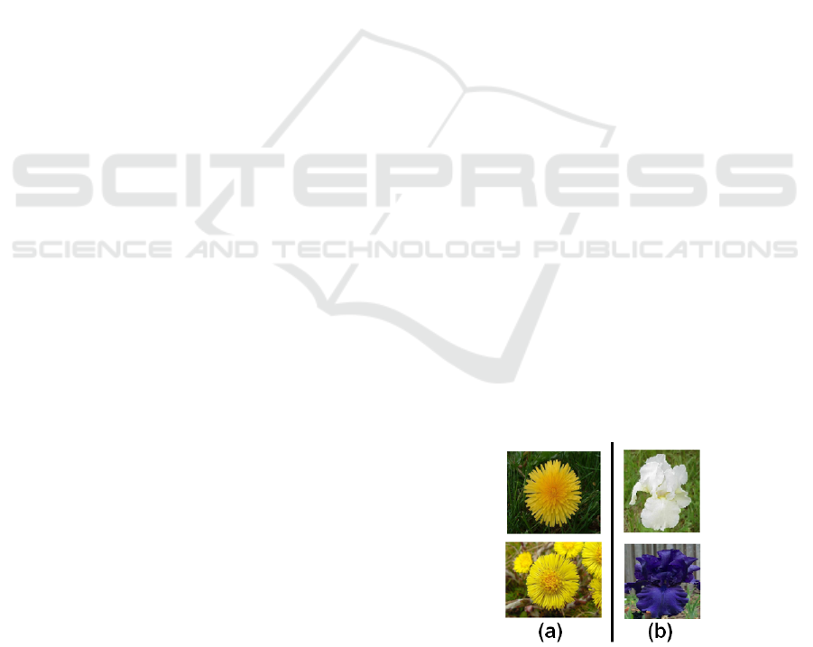
flowers from different species may seem similar, for
example Dandelion and Colt’s Foot as shown in Fig-
ure 1.a. Furthermore, flowers from the same species
may have different appearance, for example the Pansy
flower in Figure 1.b.
Figure 1: (a) Two visually dissimilar flowers from the same
species. - (b) Two visually similar flowers from different
species.
Some previous works are interested on flower clas-
sification, for example Guru and al in (Guru et al.,
2010) proposed a method to classify flowers based
on texture features. First, they used a threshold-
based method to segment the flower image. Then,
they chose two texture features : Gray level cooc-
currence matrix and Gabor filter response to describe
the flower. Finally, they classified flowers using the
k-nearest neighbor algorithm (k-NN). In (Nilsback
and Zisserman, 2008), the authors used a flower seg-
201
Ben Mabrouk A., Najjar A. and Zagrouba E..
Image Flower Recognition based on a New Method for Color Feature Extraction.
DOI: 10.5220/0004636302010206
In Proceedings of the 9th International Conference on Computer Vision Theory and Applications (VISAPP-2014), pages 201-206
ISBN: 978-989-758-004-8
Copyright
c
 2014 SCITEPRESS (Science and Technology Publications, Lda.)

mentation algorithm based on the minimization of
Markov Random Fields using graph-cuts to extract
flower from its background. Then, they describe dif-
ferent aspects of the flowers (color, shape and tex-
ture) using HSV color space, Histogram of Gradi-
ent Orientation (HOG) and SIFT descriptors. Finally,
they combined these features using a multiple ker-
nel framework with a SVM classifier. Although cited
works give good performances, they have high com-
putational complexity. In this paper, the aim is to cre-
ate an automatic flower classification system which
gives good classification rates while minimizing the
processing time. The rest of the paper is organized as
follows : in section 2, we present the different parts of
our proposed method and, in section 3, experiments
and results are provided. Finally, some conclusions
and perspectives of this work are given.
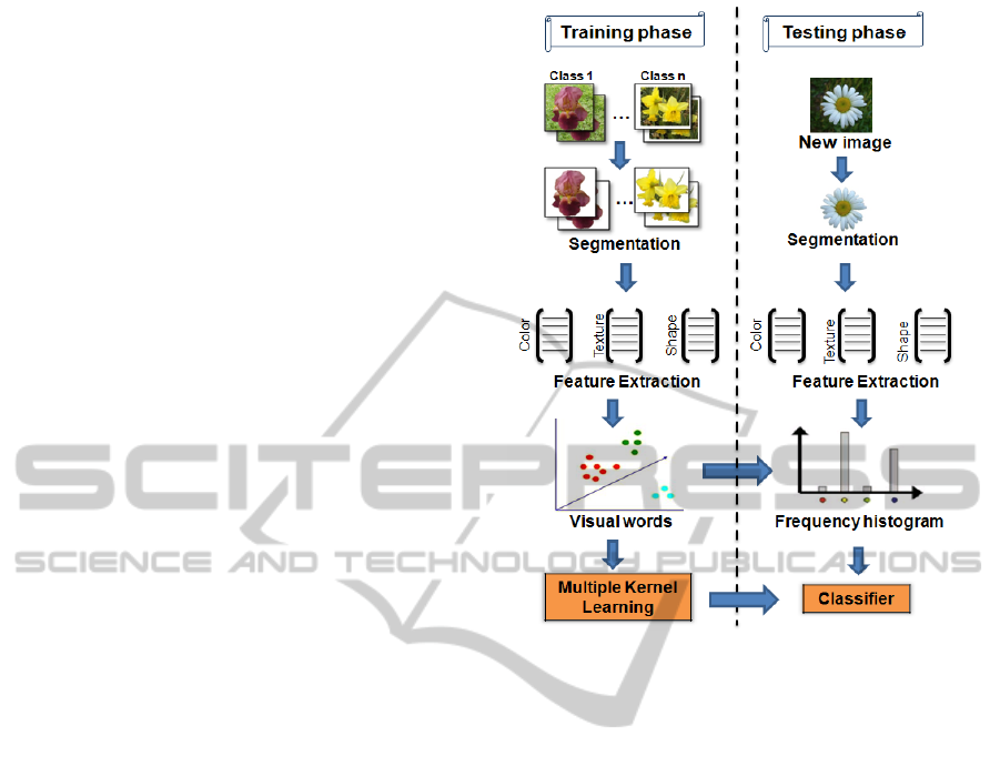
2 PROPOSED METHOD
The proposed method for flower image classification
has two phases which are the training phase and the
testing phase. The schema of this method is given in
Figure 2. The training phase aims to build a model
based on a subset of images called training images.
First, those images are segmented and the features are
extracted. Then, a visual vocabulary is computed for
each feature. Finally, for every image on training set,
we compute an histogram counting the occurrence of
each visual vocabulary word. Those histograms are
used as an input to the SVM classifier. Given the com-
puted model and the histogram of visual word of an
image, the goal of the testing phase is to identify the
class of the flower contained in this image. The differ-
ent steps of our proposed schema are detailed in the
following subsections.
2.1 Segmentation
Segmentation is an important step in an image anal-
ysis process. Generally, flowers live in similar en-
vironments and for this reason they often have sim-
ilar backgrounds. The segmentation aims to sepa-
rate the region that contains the flower (foreground)
from its background to improve the classification. In
the literature, several papers (Nilsback and Zisser-
man, 2007)(Najjar and Zagrouba, 2012) have pro-
posed segmentation algorithms. We used the segmen-
tation results obtained by the authors in (Najjar and
Zagrouba, 2012) because there method was tested and
validated on the same flower dataset that we will use
to evaluate our classification schema. The proposed
segmentation method is achieved using OTSU thresh-
Figure 2: Schema of the proposed method.
olding technique on Lab color space. The threshold-
ing was performed, separately, on the three compo-
nent L, a and b, and then the best result is chosen rel-
atively to the ground truth.
2.2 Feature Extraction
Within the same species, flowers may look very dif-
ferent and sometimes flowers from different species
may look very similar. Besides, some flowers are dis-
tinguishable by their color, others have very distinc-
tive texture or shape. The major challenge of classifi-
cation is to find suitable features to describe the visual
content of flower image and to build a classifier able
to differentiate between species. In this paper, three
features are used to represent different properties of
the flower : SURF sampled both on the foreground
region of the flower and its boundary and the Lab val-
ues.
2.2.1 Speed Up Robust Feature
SURF (Bay et al., 2008) is an interest point detector
and descriptor. First, it detect interest points based on
a approximation of the Hessian matrix determinant.
Then, around each interest point, a window is divided
into 16 sub-regions and 4 Haar wavelets responses are
VISAPP2014-InternationalConferenceonComputerVisionTheoryandApplications
202

calculated from each sub-region using the integral im-
ages. The resulting SURF descriptor is a vector of
length 64 describing the neighborhood intensity dis-
tribution.
Comparison between SURF and SIFT: SURF is in-
spired by the SIFT descriptor (Low, 2004) but it is
faster and more robust against image transformations
than SIFT (Juan and Gwun, 2009) (Bay et al., 2008).
Although SIFT features performed well in many ap-
plications such as object recognition, it has a high
computation cost. In order to reduce the feature com-
puting time, SURF use integral images to detect and
describe interest points. Moreover, SURF is more
compact than SIFT since it uses only 64 information
to describe the interest point, while SIFT uses 128.
For those reasons, we chose the SURF to extract fea-
tures from flower images. In fact, the set of SURF
interest points detected in the image is divided into
two subsets : the first one, denoted E
R
SU RF
, includes
the interest points sampled on the foreground region.
The second subset, denoted E
C
SU RF
, contains the inter-
est points computed on the boundary of the flower.
SURF on the Foreground Region: By computing
SURF features over the foreground flower region, we
can describe not only the local shape of the flower
(for example thin petal structure, flower corolla, ...),
but also its texture.
SURF on the Foreground Boundary: Flowers can
deform in different ways, and consequently the diffi-
culty of describing the flower shape is increased by
its natural deformations. Also, the petals are often
flexible and can twist, bend, ..., which changes the
appearance of the flower shape. By computing SURF
features on this area, we give more emphasis to the
local shape of the flower boundary. In fact, to extract
the boundary from an image, we converted it, first,
into binary image. Then, we perform erosion opera-
tion. Finally, we subtract the binary image from the
eroded one and the boundary is extracted.
2.2.2 Lab Values
To represent the color of the flower, we have to choose
an appropriate color space. In fact, this choice is an
important decision because it can affect the classifi-
cation result. Hence, three color spaces were stud-
ied in order to select the best one. Colors, in the
RGB space, are represented using three components
(Red, Green and Blue) which are strongly correlated.
Therefore, we didn’t choose it. Also, in the HSV
color space, three components are used to represent
the color : Hue, Saturation and Value. These spaces
are device-dependent and thereby they can influence
the color representation. However, Lab color space,
proposed by the CIE (international Commission on
Illumination) is independent of any system and it is
perceptually uniform. In addition, it is more robust
against illumination variations than RGB and HSV
color spaces. For this reason, we choose the Lab color
space to describe the color. However instead of using
all image pixels to describe the color of the flower, we
only consider a m x m window around each detected
point of interest p. This window, called ”patch”, is
selected as it is given in Equation 1.
V (p) = {q(z,t) ∈ N
2
/z ∈ [x −
m
2
,x +
m
2
]
and t ∈ [y −
m
2
,y −
m
2
]} (1)
Where (x,y) are the coordinates of p in the image and
(z,t) are the coordinates of the pixel q in the neighbor-
hood of p. This allows us to reduce both the process-
ing time and the vector dimension used to create the
color feature. First, we detect SURF interest points
on the foreground region and we obtain E
R
SU RF
. Then,
for each interest point p, we extract Lab values of its
neighbors denoted V
Lab
(p). Figure 3 shows our pro-
posed method to extract color feature.
Figure 3: Color feature extraction.
Due to the fact that there is overlapping patchs,
we obtain, for an image I, a color descriptor V
Lab
(I)
which contains redundant values. So, to cope with re-
peated values, we apply a filtering algorithm to obtain,
finally, a more compact color descriptor V
∗
Lab
(I). The
complete algorithm of the proposed feature extraction
method is summarized in Algorithm 1.
2.3 Visual Vocabulary Computing
We compute three visual vocabularies, one for each
feature d. A visual vocabulary for a feature d is cre-
ated as follows : first, d is extracted from each train-
ing image. Then, the obtained set of features is di-
vided into homogenous clusters using K-means algo-
rithm in order to obtain visual words. In fact, every
obtained cluster center is a visual word. The num-
ber K of clusters represent the size of the vocabulary
ImageFlowerRecognitionbasedonaNewMethodforColorFeatureExtraction
203

and it is sought experimentally. The next step is to
compute, for each image I, a K dimensional normal-
ized frequency histogram that counts the occurrence
of each visual vocabulary word in I.
Algorithm 1: Color feature extraction.
Input : Image I
V
Lab
(I) ← φ
E
R
SU RF
← detect SURF points(I)
for each interest point p in E
R
SU RF
do
V
Lab
(p) ← φ
V (p) ← Extract patch(
m
2
)
for each q in V (p) do
V
Lab
(q) ← Extract feature color(q)
V
Lab
(p) ← V
Lab
(p) ∪V
Lab
(q)
end for
V
Lab
(I) ← V
Lab
(I) ∪V
Lab
(p)
end for
V
∗
Lab
(I) ← Filtering algorithm(V
Lab
(I))
Output : V
∗
Lab
(I)
2.4 Multiple Kernel Learning
The learning process is performed using a multiple
kernel framework with a SVM classifier (Louradour
et al., 2007). SVM is a discriminative classifier that
learn a decision boundary that maximizes the margin
between classes. We use a weighted linear combina-
tion of kernels, with one kernel for each feature. So,
the final kernel has the form given by the Equation 2.
K(x,x
i
) =
∑
d∈D
β
d
k
d
(x,x
i
) (2)
Where x is the support vector, x
i
is the training sam-
ple, β
d
is the weight of feature d and k
d
is a Gaussian
kernel for d. The kernel weights β
d
are determined,
experimentally, and these experimentations are pre-
sented in the following section.
3 EXPERIMENTATIONS
In this section, we introduce, first, the flower dataset
and the performance measures used to evaluate our
proposed method. Then, we present the experimen-
tation results. Finally, a comparison between our
method with a previous work is performed.
3.1 Dataset and Performance Measures
Our classification system was evaluated using the
flower dataset provided by Oxford University. There
were 17 classes in this dataset. We just used 13 classes
to evaluate our proposed method because segmenta-
tion results for the four classes : snowdrops, lily of
the valleys, cowslips and bluebells are not available.
In fact, this dataset is very challenging due to changes
of viewpoint, illumination and scale between images.
Furthermore, significant amount intra-class variabil-
ity and small inter-class variability makes the dataset
more interesting. In other hand, this dataset was used
by several works in the literature (Nilsback and Zis-
serman, 2008)(Chai et al., 2011).
We divided this dataset into a training set and a test
set. We considered three different training and test set
splits. For each split, we applied the SVM classifier
using 30 images per class for training and 15 images
per class for testing. The final performance of our
method is averaged over those obtained by the three
data splits. For the performance evaluation, we mea-
sure for each flower class a recognition rate (RR) as
the proportion of correctly classified images, and to
obtain the final performance, we average the recogni-
tion rate over 13 classes (ARR).
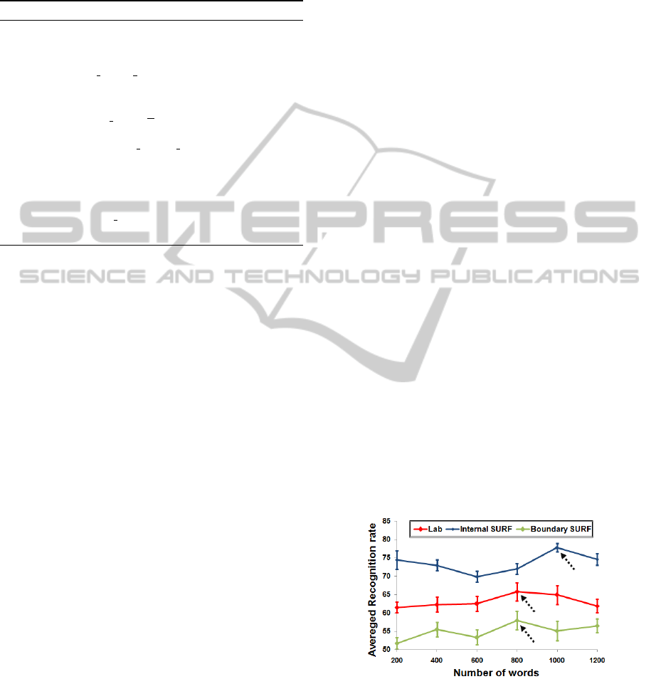
3.2 Optimization of Vocabulary Sizes
In this subsection, we aim to determine, for each fea-
ture, the optimum number of visual words in the vo-
cabulary. The classifier is trained using a single fea-
ture at time and the optimum vocabulary size is deter-
mined by varying the number of words over the range
between 200 and 1200. Then, we choose as num-
ber of words the one that gives the maximum ARR.
As given in Figure 4, the optimum number of words
is 800 for the Lab feature, 1000 for the SURF over
the foreground region and 800 for the SURF on the
boundary of the flower.
Figure 4: Vocabulary size optimization for each feature.
The pointed values are the maximum ARR.
3.3 Experimentation Results
In this subsection, we evaluate, first, the performances
of our classification method using a single feature, at
VISAPP2014-InternationalConferenceonComputerVisionTheoryandApplications
204

time. Then, we combine all the features in order to
enhance the obtained results.
Table 1: Confusion matrixes for the three features: Lab,
SURF internal and SURF boundary.
Lab
Buttercup Colt’s Foot Crocus Daffodil Daisy Dandelion Fritillary Iris Pansy Sunflower TigerLily Wild Tulip Windflower
Buttercup 60 2,22 0 11,11 0 15,56 0 0 0 0 0 11,11 0
Colt’sFoot 4,76 66,67 0 4,76 0 4,76 0 0 2,38 11,9 2,38 2,38 0
Crocus 0 0 44,44 0 4,44 0 6,67 15,56 15,56 0 0 0 13,33
Daffodil 8,89 4,44 0 57,78 0 11,11 0 2,22 0 4,44 0 11,11 0
Daisy 0 0 4,44 0 77,78 0 0 11,11 0 0 0 0 6,67
Dandelion 17,78 0 0 2,22 0 57,78 0 0 0 22,22 0 0 0
Fritillary 0 0 0 0 0 0 91,11 8,89 0 0 0 0 0
Iris 0 0 6,67 0 0 0 4,44 48,89 13,33 0 4,44 0 22,22
Pansy 0 0 13,33 0 4,44 0 0 6,67 68,89 0 0 6,67 0
Sunflower 0 13,33 0 0 0 4,44 0 0 0 82,22 0 0 0
Tigerlily 0 0 4,44 0 0 2,22 2,22 0 0 2,22 84,44 0 4,44
WildTulip 25,64 5,13 0 33,33 0 2,56 0 0 0 2,56 2,56 28,21 0
Windflower 0 0 0 0 4,44 0 0 2,22 6,67 0 0 0 86,67
SURF internal
Buttercup 66,67 0 0 2,22 0 0 8,89 13,33 2,22 0 2,22 2,22 2,22
Colt’sFoot 0 88,10 0 0 0 4,76 0 0 0 2,38 2,38 2,38 0
Crocus 0 2,22 51,11 2,22 0 4,44 0 0 8,89 0 8,89 20 2,22
Daffodil 2,22 0 13,33 57,78 0 0 0 11,11 4,44 0 2,22 8,89 0
Daisy 0 0 0 0 88,89 4,44 0 0 2,22 4,44 0 0 0
Dandelion 0 11,11 6,67 0 2,22 80 0 0 0 0 0 0 0
Fritillary 0 0 2,22 0 0 0 97,78 0 0 0 0 0 0
Iris 0 0 0 6,67 0 0 0 77,78 15,56 0 0 0 0
Pansy 2,22 0 2,22 2,22 0 0 0 0 75,56 0 2,22 0 15,56
Sunflower 0 0 0 0 4,44 0 0 2,22 0 93,33 0 0 0
Tigerlily 0 0 2,22 0 0 2,22 0 0 0 0 95,56 0 0
WildTulip 0 0 10,26 10,26 0 0 0 0 0 5,13 0 74,36 0
Windflower 8,89 0 2,22 2,22 2,22 0 0 6,67 11,11 0 2,22 0 64,44
SURF boundary
Buttercup 62,22 0 2,22 15,56 0 0 0 8,89 2,22 0 2,22 0 6,67
Colt’sFoot 0 73,81 0 0 0 21,43 0 0 0 2,38 2,38 0 0
Crocus 6,67 6,67 24,44 0 6,67 0 13,33 0 8,89 4,44 15,56 13,33 0
Daffodil 8,89 0 6,67 53,33 0 0 2,22 13,33 0 2,22 0 4,44 8,89
Daisy 0 2,22 0 0 66,67 2,22 0 2,22 6,67 0 4,44 0 15,56
Dandelion 0 13,33 0 0 15,56 46,67 0 0 0 15,56 8,89 0 0
Fritillary 0 0 0 4,44 0 0 86,67 0 2,22 0 2,22 4,44 0
Iris 13,33 0 2,22 8,89 0 0 2,22 57,78 0 2,22 6,67 0 6,67
Pansy 4,44 0 0 6,67 0 0 2,22 4,44 62,22 4,44 4,44 6,67 4,44
Sunflower 0 0 0 2,22 2,22 8,89 0 0 4,44 82,22 0 0 0
Tigerlily 0 0 17,78 2,22 2,22 2,22 15,56 6,67 8,89 2,22 37,78 4,44 0
WildTulip 5,13 0 2,56 25,64 0 0 0 0 10,26 7,69 12,82 30,77 5,13
Windflower 8,89 0 2,22 8,89 0 0 0 2,22 2,22 4,44 0 2,22 68,89
Performances using a Single Feature: Table 1
shows the confusion matrixes obtained by evaluating
the individual features and averaged over the three
data splits. The numbers along the diagonal of the
matrixes represent the recognition rate per class, and
the numbers outside this diagonal represent the er-
ror rate (misclassification rate) denoted ER. We can
see that color feature perform well for classes with
very distinguishable color such as Tigerlily (RR =
84,44%). However, this feature is not able to dis-
tinguish between flowers having the same color, like
the Wild Tulip class which is confused with the But-
tercup class (ER = 25, 64%) and the Daffodil class
(ER = 33,33%). Also, Table 1 shows that the inter-
nal SURF performs well for classes with fine petals
like Sunflower (RR = 93, 33%) and for flowers with
patterns such as TigerLily class (RR = 95, 56%). In
other hand, SURF boundary works well for classes
with particular shape f Fritillary class (RR = 86,67%).
Using a single feature to distinguish between classes
may not give good results. So, to improve the perfor-
mances, we combine the three features.
Performances for Features Combination: In order
to determine the contribution of each feature, we eval-
uate all possible combinations of two and three fea-
tures. Table 2 shows the ARR for all combinations
of two features. The number between brackets is the
weight assigned to each feature. The best result of
84,01 ± 1% is obtained by combining SURF internal
(SURF
f
) and Lab feature. Note that combining color
feature with either SURF internal or SURF boundary
(SURF
b
) leads to better performance than combining
the two SURF features. This confirms the effective-
ness of the color aspect to describe the flower.
Table 2: Recognition rates for two features combinations.
Feature 1 SURF
f
(0,6) SURF
f
(0,65) SURF
b
(0,5)
Feature 2 Lab (0,4) SURF
b
(0,35) Lab (0,5)
Recognition rate 84,01 ± 1% 69,41 ± 1,5 % 77,35 ± 2,1%
For the combination of the three features, we tested
several weighting possibilities and we chose the one
that gave the best averaged recognition rate. Indeed,
the best result of 88,07 ± 1,3 is obtained by given the
largest weight to SURF sampled on the foreground re-
gion (0,6). The weights assigned to Lab feature and
SURF sampled on the background region are respec-
tively 0,25 and 0,15.
Table 3 shows the confusion matrix for the combi-
nation of three features. By combining all the fea-
tures, we improve the classification performance for
each class. In fact, using a single feature, the classi-
fier was unable to distinguish between classes in most
cases. However, the results were enhanced when the
classification was performed by combining features
as shown in Table 3.
Table 3: Confusion matrix for the combination of three fea-
tures.
Buttercup 86,67 0 0 8,89 0 0 0 2,22 0 0 0 2,22 0
Colt’Foot 0 95,24 0 0 0 0 0 0 0 2,38 0 2,38 0
Crocus 0 0 77,78 0 4,44 0 0 0 6,67 0 0 6,67 4,44
Daffodil 0 0 0 88,89 0 0 0 4,44 0 0 0 6,67 0
Daisy 0 0 0 0 97,78 0 0 2,22 0 0 0 0 0
Dandelion 2,22 0 0 0 0 97,78 0 0 0 0 0 0 0
Fritillary 0 0 0 0 0 0 100 0 0 0 0 0 0
Iris 0 0 6,67 0 0 0 0 71,11 6,67 0 4,44 0 11,11
Pansy 0 0 2,22 2,22 0 0 2,22 0 82,22 0 0 2,22 8,89
Sunflower 0 0 0 0 0 0 0 0 0 100 0 0 0
TigerLily 0 0 0 0 0 2,22 0 0 0 2,22 95,56 0 0
WildTulip 5,13 0 2,56 30,77 0 5,13 0 0 0 0 0 56,41 0
Windflower 2,22 0 2,22 0 0 0 0 0 0 0 0 0 95,56
For example, the RR achieved, by the dandelion
class, when we used the Lab feature is of 57,78 % ,
the RR is of 80 % when we used the internal SURF
ImageFlowerRecognitionbasedonaNewMethodforColorFeatureExtraction
205

and when we used the SURF boundary, the RR is of
46,67 %. When combining all features, the RR for the
dandelion class was enhanced and is of 97,78 %.
3.4 Comparison with a Previous Work
In this subsection, we compare our work to the clas-
sification method that was proposed by Nilsback and
Zisserman in (Nilsback and Zisserman, 2008). Since
the experimental results of this method for 13 classes
are not available, we have implemented it. Table 4
shows a comparison between our method and the im-
plementation of the method proposed in (Nilsback
and Zisserman, 2008). In (Nilsback and Zisserman,
Table 4: Comparison of our method to our implementation
of Nilsback’s method.
Our method Our implementation of
Nilsback’s method
Features Vocabulary
size
RR
(%)
Features Vocabulary
size
RR
(%)
Lab 800 65,76 HSV 1100 60,96
SURF
f
1000 77,8 SIFT
f
1500 72,47
SURF
b
800 57,96 SIFT
b
1500 56,87
Lab + SURF
f
+ SURF
b
— 88,07 HSV + HOG +
SIFT
f
+ SIFT
b
— 85,08
2008), the authors used four features to describe the
flowers which are HSV values, HOG and SIFT sam-
pled both on the foreground region and its bound-
ary. This method uses a SVM classifier and gives a
recognition performance of 85,08 %. Using the same
classifier as used in (Nilsback and Zisserman, 2008),
we have combined only three features and we have
reached a recognition performance of 88,07 %. In
other hand, the construction of each vocabulary using
the K-means algorithm is a time consuming. In fact,
the complexity of this algorithm is O(T*N*M) where
T is the vocabulary size (number of visual words), N
is the dimension of the feature and M is the number of
detected points. In table 4, we can see that our method
uses not only a fewer number of features and a small
vocabulary sizes but also a more compact descriptors
than (Nilsback and Zisserman, 2008). Besides, our
method achieve better recognition rate than the im-
plementation of (Nilsback and Zisserman, 2008) and
this either using a single feature or when combining
all features.
4 CONCLUSIONS
In this paper, we proposed a new method to ex-
tract color features based on SURF interest points.
We have combined features using a multiple kernel
framework with a SVM classifier. The experimen-
tal results have proved that combining features per-
form better than using a single feature for classifica-
tion. Moreover, we have proved that our method has
achieved better results within shorter execution-time
than our implementation of the method proposed in
(Nilsback and Zisserman, 2008). As future work, we
will prove the efficiency of our method, not only, on
other types of datasets (for example mushrooms, cars,
etc), but also on datasets with a larger numbers of
classes and observations per classe. Moreover, we
will attempt to improve the performances within a
shorter execution time.
REFERENCES
Abdul Kadir, Lukito Edi Nugroho, A. S. P. I. S. (2011). Leaf
classification using shape, color, and texture features.
International Journal of Computer Trends and Tech-
nology, 2:225–230.
Bay, H., Ess, A., Tuytelaars, T., and Gool, L. V. (2008).
Surf: Speeded up robust features. Computer Vision
and Image Understanding (CVIU), 110:346–359.
Chai, Y., Lempitsky, V., and Zisserman, A. (2011). Bicos: A
bi-level co-segmentation method for image classifica-
tion. In IEEE International Conference on Computer
Vision, pages 2579–2586.
Guru, D. S., Sharath, Y. H., and Manjunath, S. (2010). Tex-
ture features and knn in classification of flower im-
ages. IJCA,Special Issue on RTIPPR, pages 21–29.
Juan, L. and Gwun, O. (2009). A comparison of sift, pca-sift
and surf. International Journal of Image Processing,
3:143–152.
Krishna Singh, Indra Gupta, S. G. (2010). Svm-bdt pnn and
fourier moment technique for of leaf shape. Interna-
tional Journal of Signal Processing, Image Processing
and Pattern Recognition, 3:67–78.
Louradour, J., Daoudi, K., and Bach, F. (2007). Feature
space mahalanobis sequence kernels: Application to
svm speaker verification. IEEE Transactions on Au-
dio, Speech and Language Processing, 15:2465–2475.
Low, D. (2004). Distinctive image features from scale-
invariant keypoints. International Journal of Com-
puter Vision, 60:91–110.
Najjar, A. and Zagrouba, E. (2012). Flower image segmen-
tation based on color analysis and a supervised evalua-
tion. In International Conference on Communications
and Information Technology (ICCIT), volume 2, pages
397–401.
Nilsback, M.-E. and Zisserman, A. (2007). Delving into the
whorl of flower segmentation. In Proceedings of the
British Machine Vision Conference, volume 1, pages
570–579.
Nilsback, M.-E. and Zisserman, A. (2008). Automated
flower classification over a large number of classes.
In Indian Conference on Computer Vision, Graphics
and Image Processing, pages 722–729.
VISAPP2014-InternationalConferenceonComputerVisionTheoryandApplications
206