
Image Analysis through Shifted Orthogonal Polynomial Moments
Rajarshi Biswas
1
and Sambhunath Biswas
2
1
Department of Computer Science, Saarland University, Saarbrucken, 66123, Germany
2
Machine Intelligence Unit, Indian Statistical Institute, 203, B. T. Road, Kolkata, 700108, India
Keywords:
Rotational Invariance, Discrete Disc, Illumination, Noise.
Abstract:
Image analysis is significant from the standpoint of image description. A well described image has merits
in different research areas, e.g., image compression, machine learning, computer vision etc. This paper is an
attempt to analyze graylevel images through shifted orthogonal polynomial moments, computed on a discrete
disc. This removes the difficulty of computing the moments on an analytic disc. Excellent rotational invariance
as well as illumination invariance is observed.
1 INTRODUCTION
Image analysis through moments has recently gained
a good amount of attention during the last two
decades in the community of image processing, com-
puter vision and pattern recognition, though its initi-
ation was made in 1962 when Hu (Hu, 1962) did his
pioneering work on moment invariants. Afterwards,
various works based on both non-orthogonal and or-
thogonal moments were carried out. Among the non-
orthogonal moments, some of the reported works
can be found in (Prokop and Reeves, 1992), (Reddi,
1981), (Abu-Mostafa and Psaltis, 1984). Similarly,
works based on orthogonal moments can be found
in (Teague, 1980), (Teh and Chin, 1988), (Z.L. Ping
and Sheng, 2002), (H. Ren and Sheng, 2003) and
(T. Xia and Luo, 2007). Attempts on discrete orthog-
onal moments using Chebyshev moments were made
by (P.T. Yap and Ong, 2003) and (R. Mukundan and
Lee, 2001), while Zhu et al. (H.Q. Zhu and Coatrieux,
2007) introduced a kind of orthogonal polynomials
defined on non-uniform lattice, knownas Racah poly-
nomials. A good survey of works on moments can be
found in the article of Shu et al. (H. Shu and Coa-
trieux, 2007) and (Jan Flusser and Zitova, 2009). In
the present paper,moment-basedrotational invariance
using orthogonal shifted polynomials on discrete disc
(Biswas and Chaudhuri, 1985) is proposed. Shifting
function bijectively maps the interval [0,1] to the in-
terval [−1,1]. Shifted polynomials are, therefore, or-
thogonal on [0,1], i.e.,on the unit disc. It should be
noted that it is difficult to use analytic disc because of
the pixel mapping problem on the analytic disc. On
the other hand, using discrete disc has many advan-
tages. The mapping is unique and straightforward be-
cause of the mathematical description of the discrete
disc. This makes the algorithms straightforward. Re-
sults show excellent behavior of invariance under ro-
tation and different conditions of illumination. This
facilitates significant image description through or-
thogonal shifted polynomial image moments.
Below in Section 2, we briefly discuss discrete
circles, rings and discs to help readers understand
the mapping on discrete disc. Section 3 describes
the proposed three different methods, while Section 4
demonstrates results and discussion. Finally, in Sec-
tion 5 we present our conclusion.
2 DISCRETE CIRCLE, RING AND
DISC
Consider a 2-dimensional discrete array space of m×
n points or pixels so that any point or pixel (x, y),
0 ≤ x ≤ m −1 , 0 ≤ y ≤ n −1. x, y,m,n ∈ I (set of
integers) can be mapped to the continuous real plane
by a unit square about the center point (x±
1
2
, y±
1
2
).
Also, for simplicity and convenience, let the radii of
the discrete circle, ring and disc be integer valued with
center of the unit squares.
Discrete Circle (dc)
A dc is a discrete space approximation to the circle
defined in Euclidean geometry. In the present scheme
of generation, a dc is defined as follows
411
Biswas R. and Biswas S..
Image Analysis through Shifted Orthogonal Polynomial Moments.
DOI: 10.5220/0004648004110416
In Proceedings of the 9th International Conference on Computer Vision Theory and Applications (VISAPP-2014), pages 411-416
ISBN: 978-989-758-003-1
Copyright
c
2014 SCITEPRESS (Science and Technology Publications, Lda.)

Definition 1. A dc with radius r and center (α, β) is
a set S
r
of 8-connected pixels so that each pixel (x, y)
satisfies the inequality
r−
1
2
< |
q
(x−α)
2
+ (y−β)
2
| < r+
1
2
(1)
Uniqueness of a dc under the above definition may be
easily established.
Rings and Discs
Since a pixel covers a square area in real space, a dc
has some width in real space. A ring or a disc can
therefore be generated by the union of circles of radii
r,r + 1,······ , r + m. However it is interesting to ob-
serve the following properties in connection with the
generation of a ring and a disc by the present method.
Definition 2. A discrete ring (dr) with integer radius
r
1
and r
2
, r
2
> r
1
and integer center (α, β) is given
by
R(r
1
, r
2
, α, β) =
r
2
[
r=r
1
S
r
(2)
if r
1
= 0 a discrete disc (dd) is generated. Here S
0
is
assumed to be the center pixel itself. It is easy to show
that there exist no hole or gap in the dr or dd generated
according to the definition 2. Thus, a discrete disc
(dd) with integer radius r and integer center (α,β) is
given by
D(r,α,β) =
r
[
r=0
S
r
(3)
It should be noted that when an image is mapped on
a discrete disc, the circumference of different circles
constituting the disc has different pixels of the image
mapped onto it. As this map is unique, positions of
pixels on each circle are also unique.
3 PROPOSED METHODS
We now examine three different shifted orthogo-
nal polynomials. Proposed polynomials include the
shifted Legendre and shifted Chebyshev polynomi-
als of both the first and second kind. Note that
shifted orthogonal polynomials have certain advan-
tages over their non-shifted versions. The advantages
are centered about the orthogonality on the unit inter-
val [0,1]. Below we discuss these polynomials.
3.1 Shifted Legendre Polynomial
The shifted Legendre polynomial is given by
P
∗
n
(x) = P
n
(2x−1) (4)
Here, the shifting function shifts x −→ 2x −1. This
shifting function is an affine transformation (i.e., it
preserves straight lines which means all points lying
on a straight line will lie on a line after the transfor-
mation. Ratios of distances between points lying on
a straight line will remain unaffected but it does not
necessarily preserve angles or lengths. Sets of paral-
lel lines will remain parallel to each other). The shift-
ing function is chosen to bijectively map the interval
[0,1] to the interval [−1, 1]. As a result, the shifted
Legendre polynomials are orthogonal on [0,1]. Since,
P
n
(x) =
1
2
n
[n/2]
∑
t=0
(−1)
t
n!
(n−t)!t!
(2n−2t)!
n!(n−2t)!
x
n−2t
, (5)
where [n/2] is the maximum integer in n/2, we get
P
∗
n
(x) =
1
2
n
[n/2]
∑
t=0
(−1)
t
(2n−2t)!
t!(n−t)!(n −2t)!
(2x−1)
n−2t
.
(6)
The orthogonality condition for this polynomial can
be written as
Z
1
0
P
∗
n
(x)P
∗
m
(x)dx =
1
2n+ 1
δ
nm
(7)
This orthogonality condition can be suitably changed
to
Z
1
0
p
(2n+ 1)P
∗
n
(x)
p
(2m+ 1)P
∗
m
(x)dx = δ
nm
. (8)
To show the rotational invariance behavior of a poly-
nomial, it must be converted to polar form, i.e., it must
be expressed as a function of radius r and polar an-
gle θ. Thus, it should have the form of V(r,θ) which
in turn, for invariant representation under rotation of
axes about the origin, can be explicitly written into its
radial part R
n
(r) and polar part e
imθ
(Bhatia and Wolf,
1954) as
V(r,θ) = g
1
(r)g
2
(θ) = R
n
(r)e
imθ
. (9)
Hence, we must express the shifted Legendre polyno-
mial as the product of two functions. Now, one can
observe the orthogonality of the radial part as
Z
1
0
R
n
(r)R
m
(r)rdr = δ
mn
(10)
To compute the radial part for the shifted Legendre
polynomial, we equate the integrands from equation
(8) and equation (10), i.e.,
p
(2n+ 1)P
∗
n
(x)
p
(2m+ 1)P
∗
m
(x) = R
n
(r)R
m
(r)r,
(11)
or,
R
n
(r) =
p
(2n+ 1)P
∗
n
(r)r
−1/2
,
=
p
(2n+ 1)r
−1/2
1
2
n
[n/2]
∑
t=0
(−1)
t
(2n−2t)!
t!(n−t)!(n−2t)!
×(2r−1)
n−2t
.
(12)
VISAPP2014-InternationalConferenceonComputerVisionTheoryandApplications
412

Therefore, in polar co-ordinates we finally get
V
nm
(r,θ) = R
n
(r)e
imθ
,
and since V
nm
(r,θ is orthogonal on the unit disc, we
write
Z
2π
0
Z
1
0
V
nm
(r,θ)V
pk
(r)rdrdθ = δ
npmk
. (13)
If we assume f(x,y) is the digital graylevel image,
then it should be suitably mapped to a discrete disc
to get f(r,θ). The Legendre moment of the image
f(x, y) can be computed by
A
P
nm
=
Z
2π
0
Z
1
0
f(r,θ)R
n
(r)e
−imθ
rdrdθ. (14)
Writing r/r
max
= ρ, we get ρ = 0 when r = 0, and
ρ = 1 when r = r
max
. Hence, A
P
nm
on the discrete unit
disc can be written as
A
P
nm
=
ρ=1
∑
ρ=0
ρR
n
(ρ)(
2π
∑
θ=0
f(ρ, θ)e
−imθ
). (15)
3.2 Normalized Shifted Legendre
Moments
To consider normalized Legendre moments A
L
nm
, we
must normalize f (ρ,θ), R
n
(r) and e
−imθ
. We normal-
ize f(ρ,θ) by dividing it by the square root of the sum
of its elements, i.e., the normalized value
˜
f(ρ,θ) is
˜
f(ρ, θ) =
f(ρ, θ)
v
u
u
t
ρ=1
∑
ρ=0
2π
∑
θ=0
[ f(ρ,θ)]
2
, (16)
so that
ρ=1
∑
ρ=0
2π
∑
θ=0
[
˜
f(ρ, θ)]
2
= 1 (17)
Similarly, we normalize R
n
(ρ) by dividing it by the
square root of the product of the maximum value of
n, i.e., r
max
and the sum of the squired valuesof R
n
(ρ).
˜
R
n
(ρ) =
R
n
(ρ)
r
r
max
∑
ρ∈D
[R
n
(ρ)]
2
, (18)
where D is the discrete unit disc. Finally, |e
−imθ
| = 1.
Hence, the normalized shifted Legendre moments is
given by
˜
A
P
∗
nm
=
ρ=1
∑
ρ=0
ρ
˜
R
n
(ρ)(
2π
∑
θ=0
˜
f(ρ, θ)e
−imθ
). (19)
3.3 Invariance and Illumination
It should be noted that equation (19) holds good, in
general, for all shifted orthogonal polynomials.
3.3.1 Invariance
When a graylevel image f(ρ,θ) rotates about a point
by an angle α, it becomes noisy and blurred to some
extent. Normalized moments are capable of handling
this situation. To observe this, we consider
g(ρ,θ + α) = f(ρ, θ+ α) + n(ρ,θ + α) (20)
Therefore,
˜
A
L(g)
nm
=
ρ=1
∑
ρ=0
ρ
˜
R
n
(ρ)(
2π
∑
θ=0
˜g(ρ,θ+ α)e
−im(θ+α)
),
=
ρ=1
∑
ρ=0
ρ
˜
R
n
(ρ)(
2π
∑
θ=0
˜
f(ρ,θ+ α)e
−im(θ+α)
)
+
ρ=1
∑
ρ=0
ρ
˜
R
n
(ρ)(
2π
∑
θ=0
˜n(ρ, θ+ α)e
−im(θ+α)
)
≈
˜
A
L( f(θ+α))
nm
.
(21)
L in equation (21), is used for P
∗
to indicate the valid-
ity of the equation for all shifted polynomials. since,
the orthogonal moments
˜
A
nm
can be viewed as the
correlation between the image and the moment kernel
(Yap and Raveendran, 2004), the second term is zero
because the correlation of the low spatial frequency
moment kernel and the high spatial frequency of the
noise is small. In other words, when n and m in
˜
A
nm
are low,
ρ=1
∑
ρ=0
ρ
˜
R
n
(ρ)(
2π
∑
θ=0
˜n(ρ, θ)e
−imθ
) ≈ 0 (22)
Therefore,
˜
A
L( f(θ+α))
nm
=
ρ=1
∑
ρ=0
ρ
˜
R
n
(ρ)(
2π
∑
θ=0
˜
f(ρ, θ+ α)×
e
−im(θ+α)
)
= Tr(α)
ρ=1
∑
ρ=0
ρ
˜
R
n
(ρ)(
2π
∑
θ=0
˜
f(ρ,θ)×
e
−im(θ+α)
)
=
ρ=1
∑
ρ=0
ρ
˜
R
n
(ρ)(
2π
∑
θ=0
Tr(α)
˜
( f)(ρ, θ)×
e
−im(θ+α)
)
=
˜
A
L(Tr(α) f (θ))
nm
e
−imα
(23)
where Tr(α) is the rotational transformation on the
image in the discrete domain. Thus,
|
˜
A
L( f(θ+α))
nm
| ≈ |
˜
A
L( f(θ))
nm
| (24)
ImageAnalysisthroughShiftedOrthogonalPolynomialMoments
413

3.4 Illumination
When the illumination changes by a factor of c, the
new image g(x, y) = cf(x,y). In polar co-ordinates
g(ρ,θ) = cf(ρ, θ). Now,
˜g(ρ,θ) =
c
˜
f(ρ, θ)
v
u
u
t
ρ=1
∑
ρ=0
2π
∑
θ=0
|cf(ρ,θ)|
2
=
˜
f(ρ,θ) (25)
Thus, under illumination change
˜
A
L(g)
nm
=
ρ=1
∑
ρ=0
ρ
˜
R
n
(ρ)(
2π
∑
θ=0
˜g(ρ,θ) ˜e
−imθ
),
=
˜
A
L( f)
nm
.
(26)
It is already established that moments can serve well
as features. From the computational point of view,
low order normalized moments can be computed very
quickly and hence the high order normalized mo-
ments can be easily obtained. We consider the ratio
of high to low order moments as our feature. Low
order moment is chosen as M
l
=
s
(
N−1
∑
n=0
M− 1
∑
m=0
|
˜
A
nm
|
2
,
while the high order moment is M
h
= 1 − M
l
. M
l
and M
h
correspond to the low spatial frequency (low-
pass) and high spatial frequency (high-pass) compo-
nents of the image. The ratio of these two moments,
R
M
= M
h
/M
l
can be taken as an effective feature.
To consider this ratio feature of moments for other
orthogonal polynomials, we simply consider the un-
derlying polynomials and their radial form. Compu-
tation of moments for them is self explanatory.
3.5 Shifted Chebyshev Polynomial of
First Kind
Shifted Chebyshev polynomial of the first kind is
defined by T
∗
n
(x) = T
n
(2x − 1), where T
n
(x) is the
Chebyshev polynomial of the first kind and is de-
scribed by
T
n
(x) =
n
2
[n/2]
∑
t=0
(−1)
t
(n−t −1)!
t!(n−2t)!
(2x)
n−2t
. (27)
Hence,
T
∗
n
(x) = T
n
(2x−1),
=
n
2
[n/2]+1
∑
t=0
(−1)
t
(n−t −1)!
t!(n−2t)!
×[2(2x−1)]
n−2t
.
(28)
The orthogonality condition is
Z
1
0
(x−x
2
)
−1/2
T
∗
n
(x)T
∗
m
(x)dx =
π
2
δ
nm
,n 6= 0
= πδ
nm
,n = 0
(29)
Therefore, in the polar form, the radial polynomial
can be written as
R
n
(r) =
√
π(r−r
2
)
−
1
4
r
−
1
2
n
2
[n/2]+1
∑
t=0
(−1)
t
×
(n−t−1)!
t!(n−2t)!
[2(2r−1)]
n−2t
, for n = 0.
(30)
It should be noted that the shifted Chebyshev polyno-
mial of the first kind is orthogonal on the interval[0,1]
with respect to the weight function w(x) = (x−x
2
)
−
1
2
.
In the polar form this becomes w(ρ) = (ρ −ρ
2
)
−
1
2
.
Obviously, when ρ = 1, w(ρ) becomes infinite. It
is therefore, clear that on the unit discrete disc, the
shifted Chebyshev polynomial moments of first kind
on the circumference are undefined and hence cannot
be used for recognition features. However, one can
easily get over this problem by computing the mo-
ments on a discrete unit ball because a ball does not
consider its circumference. To enhance accuracy, one
can consider the value of ρ = r
max
/(r
max
+ 1) when
r = r/r
max
= 1.
3.6 Shifted Chebyshev Polynomial of
Second Kind
Shifted Chebyshev polynomial of second kind, U
∗
n
is
free from any kind of computational problem because
it is orthogonal on the interval [0,1] with respect to
the weight function w(x) = (x−x
2
)
1
2
. And,
U
∗
n
(x) = U
n
(2x−1),
=
[n/2]+1
∑
t=0
(−1)
t
(n−t)!
t!(n−2t)!
×[2(2x−1)]
n−2t
.
(31)
U
n
(x) is the shifted Chebyshev polynomial of second
kind. The corresponding radial polynomial can be
computed as
R
n
(r) = U
∗
n
(r)r
−1/2
=
p
8/π(
1−r
r
)
1
4
[n/2]+1
∑
t=0
(−1)
t
(n−t)!
t!(n−2t)!
×[2(2r −1)]
n−2t
,
(32)
4 EVALUATION OF THE MERIT
OF THE WORK
Almost all the authors have computed moments of
Chebyshev polynomials on a rectangle. Ping et
al. (Z.L. Ping and Sheng, 2002) introduced shifted
VISAPP2014-InternationalConferenceonComputerVisionTheoryandApplications
414
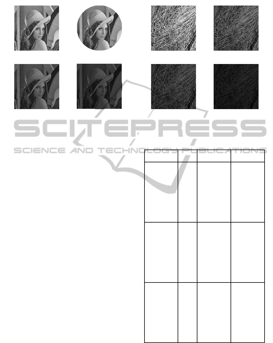
(a) (b)
(c) (d)
Figure 1: (a) Lena image, c = 1.0 (b) Map on the discrete
disc (c)Lena image, c = 0.6 (d)Lena image, c = 0.4.
Chebyshev polynomial moment of the second kind
on an analytic disc. As the discrete points or pixels
are defined on a rectangular grid, this needs a spe-
cial mapping technique to find the pixel position on
a disc. One of the solutions is to use a polar raster.
The problems with the polar raster and the errors of
the reconstruction are analyzed in detail in (Mikola-
jczyk and Schmid, 2004). Our method uses a dis-
crete disc for unique mapping of pixels. As a result,
computation in our case becomes easy and straight-
forward, and removes the difficulty of mapping pix-
els on an analytic disc. Besides, in addition to ex-
amining shifted Chebyshev polynomial of the second
kind, we have also examined the feasibility of us-
ing the shifted Chebyshev polynomial of first kind
and shifted Legendre polynomial. Result shows all
of them are equally efficient.
5 RESULTS AND DISCUSSION
Fig. 1 shows the Lena image and its map on a discrete
disc, while Fig. 2 shows the straw image at differ-
ent illuminations. Table 1 describes the result of rota-
tional invariance with θ = 0 and varying α in equation
(24), while Table 2 describes the result of illumination
invariance with varying c in equation (25).
6 CONCLUSIONS
Image description through moments of orthogonal
shifted polynomials has been proposed. This descrip-
tion is rotationally invariant as well as illumination
(a) (b)
(c) (d)
Figure 2: (a)Straw image, c = 1 (b)Straw image, c = 0.6
(c)Straw image, c = 0.4 (d)Straw image, c = 0.2.
Table 1: Rotational Invariance for Lena Image, N = M = 6.
Polynomial Image Value of R
M
α in eqn.(24)
0
o
1.556585e+2
30
o
1.555999e+2
60
o
1.552167e+2
Shifted 90
o
1.556327e+2
Legendre Lena 120
o
1.556154e+2
150
o
1.552846e+2
180
o
1.556736e+2
210
o
1.553731e+2
240
o
1.554150e+2
270
o
1.555708e+2
0
o
6.023204e+1
30
o
6.025693e+1
60
o
6.004949e+1
Shifted 90
o
6.033060e+1
Chebysheb Lena 120
o
6.035521e+1
First Kind 150
o
6.011921e+1
180
o
6.030006e+1
210
o
6.007316e+1
240
o
6.006964e+1
270
o
6.016374e+1
0
o
1.981176e+1
30
o
1.976791e+1
60
o
1.974387e+1
Shifted 90
o
1.974037e+1
Chebysheb Lena 120
o
1.972534e+1
Second Kind 150
o
1.972488e+1
180
o
1.977120e+1
210
o
1.978165e+1
240
o
1.980989e+1
270
o
1.981933e+1
invariant. Therefore, it can be used in many appli-
cations, such as, compression, computer vision and
recognition purposes. We have investigated the in-
ImageAnalysisthroughShiftedOrthogonalPolynomialMoments
415

Table 2: Illumination Invariance for textured images, N = M = 6.
Polynomial Image Value of c R
M
Image Value of c in eqn.(25) R
M
Shifted 1.0 1.819310e+2 1.0 1.556327e+2
Legendre 0.8 1.811447e+2 0.8 1.551542e+2
Straw 0.6 1.799795e+2 Lena 0.6 1.544699e+2
0.4 1.782080e+2 0.4 1.536190e+2
0.2 1.765312e+2 0.2 1.547770e+2
Chebysheb 1.0 7.114174e+1 1.0 6.023204e+1
First Kind 0.8 7.058486e+1 0.8 5.985514e+1
Straw 0.6 6.972407e+1 Lena 0.6 5.929079e+1
0.4 6.825735e+1 0.4 5.837455e+1
0.2 6.548399e+1 0.2 5.715533e+1
Shifted 1.0 1.974037e+1 1.0 1.981176e+1
Chebysheb 0.8 1.972534e+1 0.8 1.986103e+1
Second Kind Straw 0.6 1.972488e+1 Lena 0.6 1.996325e+1
0.4 1.981933e+1 0.4 2.023949e+1
0.2 1.981933e+1 0.2 2.160718e+1
variance through computation of global moments of
images. For invariance, we have computed the ratio
features of moments. It is found that the computa-
tion of invariance through ratio of moments over lo-
cal subimages is more powerful than that computed
computed over the entire image. Such features can be
used in correspondence problem. Our future work is
based on such local invariance of patches in images.
REFERENCES
Abu-Mostafa, Y. and Psaltis, D. (1984). Recognitive as-
pects of moment invariants. IEEE Trans Pattern Anal.
Machine Intell., 6:698–706.
Bhatia, A. B. and Wolf, E. (1954). On the circular polyno-
mials of zernike and related orthogonal sets. In Proc.
Cambridge Philosos. Soc. 50.
Biswas, S. N. and Chaudhuri, B. B. (1985). On the genera-
tion of discrete circular objects and their properties.
Comput. Vision, Graphics Image Process., 32:158–
170.
H. Ren, Z. Ping, W. B. W. W. and Sheng, Y. (2003). Multi-
distortion invariant image recognition with radial har-
monic fourier moments. J. Opt. Soc. Am. A, 20:631–
637.
H. Shu, L. L. and Coatrieux, J. L. (2007). Moment-
based approaches in image. In IEEE Engineering in
Medicine and Biology Magazine.
H. Q. Zhu, H. Z. Shu, J. L. L. L. and Coatrieux, J. (2007).
Image analysis by discrete orthogonal racah moments.
Signal Processing, 87:687–708.
Hu, M. (1962). Visual pattern recognition by moment in-
variants. IRE Trans. Inform. Theory IT, 8:179–187.
Jan Flusser, T. S. and Zitova, B. (2009). Moments and Mo-
ment Invariants in Pattern Recognition. John Wiley
and Sons, UK.
Mikolajczyk, K. and Schmid, C. (2004). Scale and affine in-
variant interest point detectors. International Journal
of Computer Vision, 60:63–86.
Prokop, R. and Reeves, A. (1992). A survey of moment-
based techniques for unoccluded object representation
and recognition. CVGIP: Graphical Models and Im-
age Process., 54:438–460.
P. T. Yap, R. P. and Ong, S. (2003). Image analysis by
krawtchouk moments. IEEE Trans. Image Process.,
12:1367–1377.
R. Mukundan, S. H. O. and Lee, P. A. (2001). Image anal-
ysis by tchebichef moments. IEEE Trans. Image Pro-
cess., 10:1357–1364.
Reddi, S. (1981). Radial and angular moment invariants for
image identification. IEEE Trans Pattern Anal. Ma-
chine Intell., 3:240–242.
T. Xia, H.Q. Zhu, H. S. P. H. and Luo, L. (2007). Image de-
scription with generalized pseudo-zernike moments.
J. Opt. Soc. Am. A, 24:50–59.
Teague, M. (1980). Image analysis via the general theory
of moments. J. Opt. Soc. Am., 70:920–930.
Teh, C. and Chin, R. (1988). On image analysis by the
methods of moments. IEEE Trans. Pattern Anal.
Mach. Intell., 10:496–513.
Yap, P. T. and Raveendran, P. (2004). Image focus mea-
sure based on chebyshev moments. In IEE Proc. -Vis.
Image Signal Process.
Z. L. Ping, R. W. and Sheng, Y. (2002). Image description
with chebyshev-fourier moments. J. Opt. Soc. Am. A,
19:1748–1754.
VISAPP2014-InternationalConferenceonComputerVisionTheoryandApplications
416
