
Experimental Comparison of Vasculature Segmentation Methods
Yuchun Ding
and Li Bai
School of Computer Science, Nottingham University, Wollaton Road, Nottingham, U.K.
Keywords: Vascular Segmentation, Retinal Vasculature, Micro-CT.
Abstract: Vessel segmentation algorithms play a very important role in vascular disease diagnosis and prediction.
Current vessel segmentation research uses mostly images of large vessels, which are relatively easy to
extract, but segmenting microvasculature is more challenging and very important for analysing vascular
disease such as Alzheimer’s Diseases. The aim of this paper is to report experimental results of several
common vessel image segmentation methods. Retinal vessel image database DRIVE is used for 2D
experiments and a micro-CT image is used for 3D experiments.
1 INTRODUCTION
Vascular pathology is present in most human
diseases, so there has been intense research in the
past in Magnetic Resonance Imaging (MRI) for
diagnosis and treatment of vascular diseases.
Recently the role of neurovascular dysfunction has
been identified, including Alzheimer's Diseases
(AD). A significant finding is that vascular
abnormalities and angiogenesis could potentially
serve as an early biomarker of the diseases. But the
lack of computational tools is becoming increasingly
apparent. A feasible way to validate the theory
linking microvasculature to pathology of
neurodegenerative conditions on large datasets is to
develop an automated computational analysis
method. However, existing algorithms for image
analysis have mostly been developed for segmenting
large vessels, and analysis of these vessels has been
limited to measuring curvature and diameter of
individual vessels, which are unsuitable for
microvasculature. Imaging devices such as micro-
CT can achieve resolutions on the order of several
μm, allowing imaging the three dimensional (3D)
microvasculature down to the capillary level. The
main weakness of using micro-CT for vascular
research is considered to be the lack of software for
3D quantification of microvasculature. Four well-
known segmentation methods were investigated,
which include local entropy thresholding (LET),
level set methods, vesselness filter, and wavelet
transform modulus maxima (WTMM). All of these
are well-performed on 2D retinal images and the aim
of this paper is to review, analyse and compare the
vessel segmentation methods in both 2D and 3D
vessel images and to show the microvasculature
detection performance of each method.
2 METHODS
2.1 Image Databases
We have chosen the retinal vessel image from a
publicly available database DRIVE (Staal et al.,
2004) for our 2D experiments because it is a
commonly used database for previous research on
vessel segmentation. The database is made up of 40
images that have been randomly selected from a
diabetic retinopathy (DR)-screening program. Each
image has a dimension of 565 by 584 pixels. For
each image in the test set, two manual segmentations
of blood vessels are available. The second set of
manual segmented image will be used in this
investigation because is it the observer results most
commonly used when comparing effectiveness of
method.
As the existing publicly available brain
vasculature dataset such as MRI, CTA or MRA
images only contain large vessels, which is not
possible for analysing the microvasculature, a
corrosion casting method was used to prepare 3-D
resin casts of the microvasculature of wild type and
transgenic Alzheimer mice model brains (Bedford et
al., 2008). The animals were lightly fixed in 4%
paraformaldehyde by transcardiac perfusion at
425
Ding Y. and Bai L..
Experimental Comparison of Vasculature Segmentation Methods.
DOI: 10.5220/0004648804250432
In Proceedings of the 9th International Conference on Computer Vision Theory and Applications (VISAPP-2014), pages 425-432
ISBN: 978-989-758-003-1
Copyright
c
2014 SCITEPRESS (Science and Technology Publications, Lda.)
120mmHg prior to delivery of fluorescent PN4 resin
via a syringe pump. After 48hr curing time, the
brains were removed and macerated in 10% KOH
for a period of 2 weeks at 37°C. The resin casts were
thoroughly washed in DDH2O and immersed in 2%
Os04 for a further 3 days then washed and freeze
dried for micro-CT (Skyscan 1174) scanning.
Measurements were obtained at a voltage of 40 kV,
current of 800 μA and voxel resolution of 24 μm.
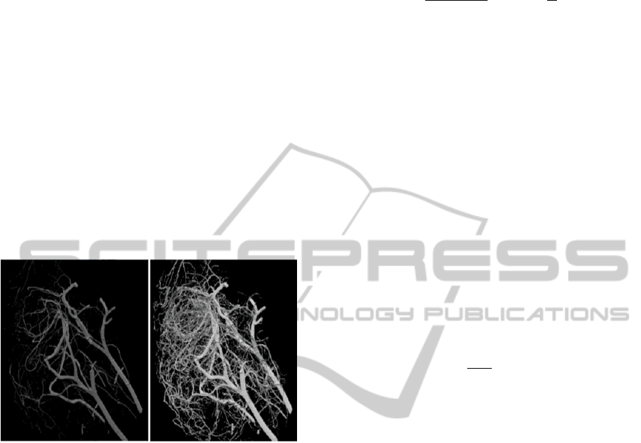
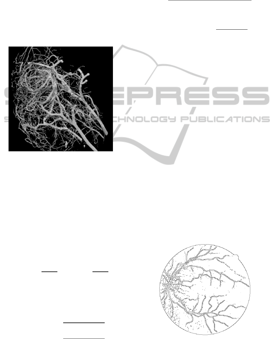
Figure 1 shows a 3D view of the original Micro-
CT scanned image of dimension 305305320
pixels visualised using MRIcron (Rorden et al.,
2007). Due to limitations of the viewer selected,
those faint and narrow vessels with low contrast are
barely visible, a simple thresholding method was
applied to reveal the vessels in the image for the
purpose of visualisation. The image on the right in
Figure 1 shows the expected resulting image.
Figure 1: Original Image (left), Enhanced Image (right).
2.2 Image Enhancement
A review of retinal blood vessel segmentation using
images from the DRIVE database has shown that
most of the vessel image segmentation algorithms
could only achieve 70% and 80% of blood-vessel
pixel are correctly classified (Fraz et al., 2012). This
is due to the difficulty of visualising small vessels in
images. As such, it is desirable to enhance the
vessels in images prior to segmentation. The paper
uses following enhancement methods.
2.2.1 Gabor Filter
The Gabor filter is a Gaussian kernel function
modulated by a sinusoidal plane wave in 2D and it is
capable of tuning a signal to specific frequencies
(Daugman, 1988). The Gabor filter that we use for
our work (blood vessel enhancement) can be
represented by:
g
,,,,
x,
y
exp
x
′
γ
y
′
2σ
cos2π
x
′
λ
φ
(1)
x
′
xcos
θ
y
sin
θ
(2)
y
′
xsin
θ
y
cos
θ
(3)
where λ is the wavelength of the cosine factor, θ
specifies the filter direction, φ is a constant
representing the phase offset, γ represents spatial
aspect ratio, with σ as the standard deviation of the
filter’s Gaussian factor.
2.2.2 Matched Filter
Matched filter convolves a signal with a designed
kernel and extracts information (from that signal)
which matches the kernel. Based on the fact that
those blood vessels are typically line-like, with small
curvatures and usually have a relatively low
contrast, a matched filter kernel was given that
matched the multiple intensity profile of the vessels’
cross section rather than a single one (Pająk, 2003):
,
2
,
|
|
/2,
(4)
Here, defines the spread of the intensity profile
and is the length of the segment. It is assumed that
a fixed vessel has orientation along the y-axis. In
reality, vessels are oriented in many different
directions, so a set of kernels is applied at each pixel
and only the maximum response is retained.
2.3 Segmentation
This section reviews four vessel segmentation
methods, and describes our own experiments with
the methods.
2.3.1 Local Entropy Thresholding
2.3.1.1 Theory
Local entropy thresholding (LET) was proposed for
segmenting retinal blood vessels (Chanwimaluang
and Fan, 2003). The key point of this method is to
automatically estimate the threshold value, based on
the entropy of an image, using a co-occurrence
matrix. A gray level co-occurrence asymmetric
matrix
is created to indicate spatial structural
information of an image – the
,
entry of the
matrix that gives the number of times the gray level j
follows the gray level i:
VISAPP2014-InternationalConferenceonComputerVisionTheoryandApplications
426
(5)
where
1
,
,1
,
1,
0
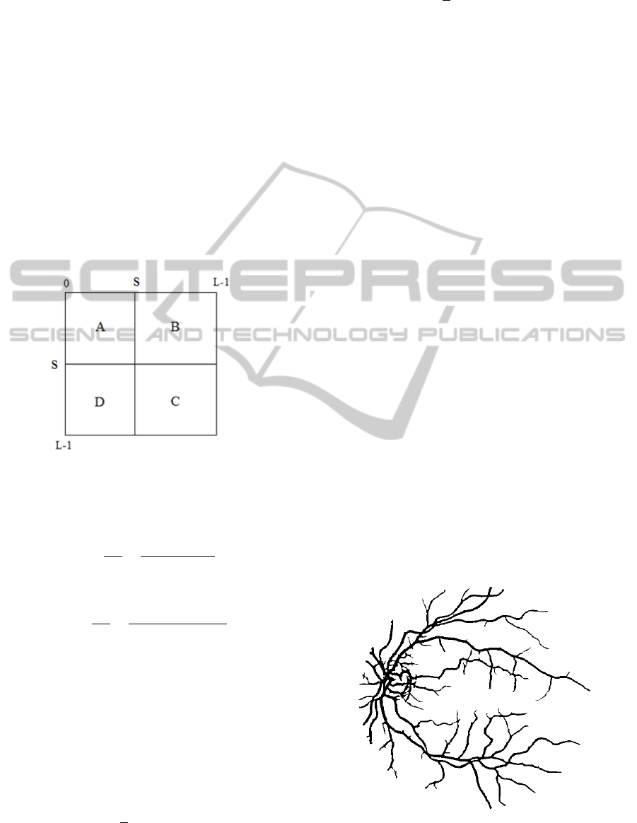
Let be the threshold such that 01.
Then threshold partitions the co-occurrence matrix
(Pal and Pal. 1989), into 4 quadrants, namely A, B,
C, and D, as shown in Figure 2, where A and C
represent gray level transition within the vessel
object and background respectively. The gray level
transition between the vessel object and background
are placed in quadrant B and D.
Figure 2: Quadrants of co-occurrence matrix.
The normalised probabilities of each quadrant are
defined as:
,
,
∑∑
(6)
0,0
,
,
∑∑
(7)
11,1
1
Where
is the probability of co-occurrence of gray
levels i and j.
and
are the probabilities of
vessel object and background.
Hence, the total second-order local entropy of the
object and background can be written as:
(8)
1
2
log
(9)
1
2
log
(10)
The gray level corresponding to the maximum of
gives the optimal threshold for vessel and
non-vessels classification. Then length filtering is
used to remove misclassified pixel.
2.3.1.2 Experiment
For testing the performance of LET, we choose
matched filter followed by Gabor filter for vessel
enhancement (Ding et al., 2013). Gabor filters
parameters are selected using a genetic algorithm
tool in MATLAB. The algorithm continually
reproduces a new generation of ‘offsprings’, which
inherit features from the previous generation and
eventually leads to an optimal solution.
The proposed method retains the computational
simplicity and straightforwardness and at the same
time achieves accurate segmentation results of
retinal images. Using a genetic algorithm can help to
find good parameters for the filter but it is also time
consuming, technically the selected value can be
only used for specific image of current interest.
Figure 4 clearly shows that LET with the Gabor
filter performed very well compared to LET, as
shown in Figure 3. More narrow vessels are detected
although few non-vessel pixels are incorrectly
classified. 3D enhancement was not implemented as
it is not sufficient to convolve all 26 directions.
Figure 5 visualised the result of LET without pre-
processing the image and many narrow vessels were
misclassified. The drawback of the LET method is
that it is not scale-invariant and does not handle
vessels of different parameters well.
Figure 3: Result of LET without Gabor Filter in 2D.
ExperimentalComparisonofVasculatureSegmentationMethods
427
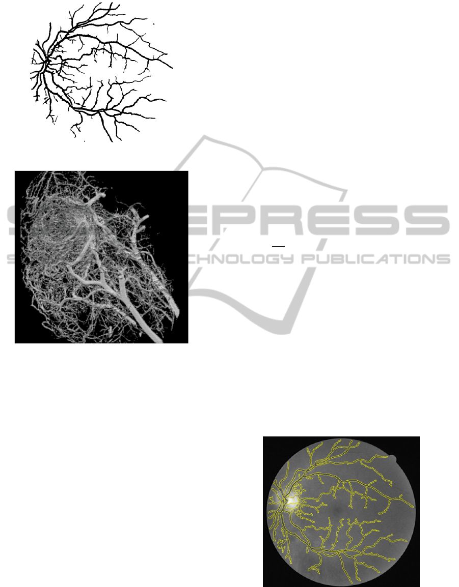
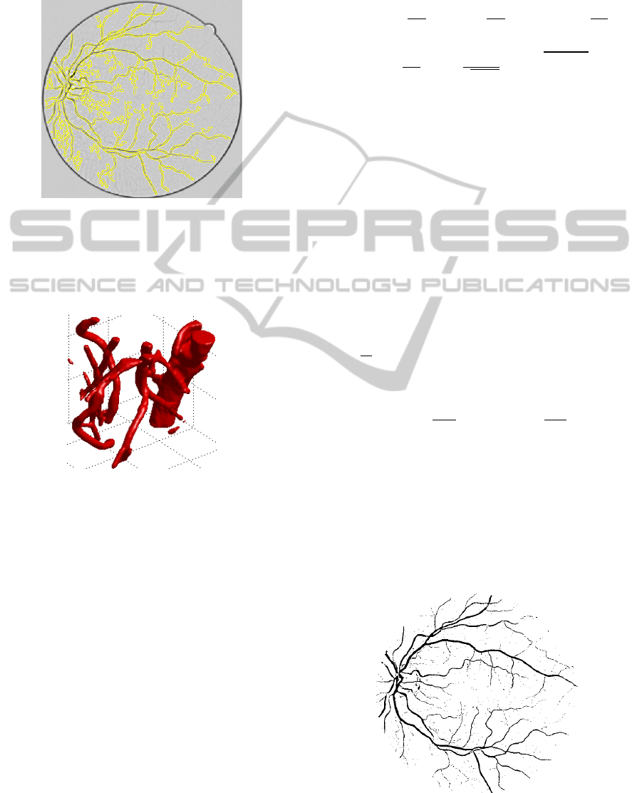
Figure 4: Result of LET with Gabor Filter in 2D.
Figure 5: Result of LET in 3D.
2.3.2 Level Set
2.3.2.1 Theory
The level set method is a powerful mathematical and
computational tool for tracking the evolution of
curves/surfaces. The basic idea of the method is to
evolve a curve by applying forces normal to the
surface and the contour evolution stops at positions
where the values of gradient magnitude are large.
This method is fast on regular image but it often
fails at low contrast edges or gaps in the object as it
is highly dependent on image contrast; as a result,
the evolving contour simply leaks through the gaps
and the object is represented by incomplete contours
in some particular fashion.
A complex level set method was introduced
based on local phase (Lathen et al., 2008). Because
vessels appear either as lines or edge pairs with
varying widths and contrasts, the method uses the
outcome of quadrature filters as a complex valued
filter pair consisting of a line filter as real part and
an edge filter as imaginary part. The filtered signal is
strongly "line-like" when the filter response is purely
real, is edge-like when it is purely imaginary. The
magnitude of the filter response gives the strength of
the structure, while the angle (local phase, the
argument of the complex value) of the response
indicates whether it is line or edge. Because it is
independent of signal strength, the local phase as a
line/edge detector is invariant to image contrast,
making it more powerful when compared to
gradient-based edge detectors. Multiscale is then
achieved using a weighted sum over all scales, and
normalisation is applied to the output. The outcome
is a "global" phase that can be used to drive a
contour robustly towards the vessel edges.
Then a level set method (Osher and Sethian,
1988) for front propagation is used to relate to the
phase based edge detector (global phase map). The
idea is to use the real part of the phase map as a
speed function. This is expressed by:
|
|
ϗ
|
|
(11)
Where denotes the normalized phase map, is a
regularisation parameter and ϗ is curvature.
2.3.2.2 Experiment
The local phase method described can distinguish
line and edge by taking local phase into account.
Most importantly, it halts the evolving contour at the
end of the vessel to prevent leakage. Although the
method succeeds in object and motion segmentation,
it fails for images that contain faint and narrow
vessel pixels, leading to the level set terminating
early and leaving many vessels undetected, as shown
in Figure 6.
Figure 6: Result of Phased Based Level Set.
In our experiment we use matched filter to enhance
vessel image before level set segmentation. Figure 7
VISAPP2014-InternationalConferenceonComputerVisionTheoryandApplications
428
shows the result image using level set with matched
filtered image, many faint vessels were detected,
although level set contour was not terminated at few
background pixels.
Figure 7: Result of our method.
We have failed to complete the experiment using 3D
images because of high computational cost. The
image shown in Figure 8 is the 3D segmentation
result after 30 minutes implementation.
Figure 8: Result of Level Set in 3D.
2.3.3 Multiscale Vesselness Filter
2.3.3.1 Theory
The multiscale second order local structure of an
image (Hessian) is examined to develop a vessel
enhancement filter (Frangi et al., 1998). A
vesselness measure is obtained from all eigenvalues
of the Hessian to determine a pixel is plate-like (Sato
et al., 1998), tubular-like or blob-like. Let
be the
eigenvalue with the k-th smallest magnitude, for an
ideal tubular structure in a 3D image, given as:
|
|
|
|
|
|
|
|
0,
|
|
≪
|
|
,
(12)
The vesselness function is then defined by
probability-like estimates of vesselness according to
two geometric ratios (
) to ensure that
only the geometric information of the image is
captured:
0
0
0,
1exp
exp
1exp
(13)
where
|
|
|
|
,
|
|
|
|
,
∑
refers to the largest area cross section of the
ellipsoid, used for distinguishing between plate-like
and line like structure, while
accounts for the
deviation from a blob-like structure but cannot
distinguish between a line and a plate like pattern,
is defined using Frobenius matrix norm to control
the sensitivity of
to background noise. Here
is the dimension of the image. This measurement
will give a high value for regions with high contrast
and a low value for the background where no
structure is present. , and are thresholds which
control the sensitivity of the line filter to the
measures
,
and . The equation for 2D images
follows from the same reasoning as in 3D where
.
0
0,
exp
2
1exp
2
(14)
A final estimate of vesselness will then be integrated
with the filter responses at different scales as
vessels appearing in varying width.
2.3.3.2 Experiment
The advantages of the vesselness filter are that it is
fast, simple, and accurate, as shown in Figure 9.
Figure 9: Result of Vesselness Filter in 2D.
ExperimentalComparisonofVasculatureSegmentationMethods
429
It can also be utilised for separating arteries or
muscles from veins using specified scale values.
Figure 10 shows the 3D result that uses two different
scale values. 3D vesselness filter is a most
commonly used methods for enhancing or extracting
vasculature, although it still suffers from two major
drawbacks. It is not scale invariant: user interaction
is required for selecting the range of scales, although
it is very difficult to adjust the value; It does not
perform well on retinal images with massive amount
of lesions, therefore pre-processing is required.
Figure 10: Result of Vesselness Filter in 3D.
2.3.4 WTMM
2.3.4.1 Theory
A multiscale edge detection algorithm was
developed base on wavelet transform modulus
maxima (Mallat and Sifen, 1992). The method can
detect the irregularities (edges) in an image with
slight noise and without intensity inhomogeneity.
Suppose , is a smooth two-dimensional
differentiable function, then a two dimensional
wavelet (e.g. Gaussian) can be defined as
,
and
, where:
,
,
,
,
,
(15)
The wavelet transformation uses only two
components
,
and
,
, in
dyadic scales:
,
,
2
∗
,
∗
,
(16)
Here * expresses the convolution. Wavelet transform
modulus and gradient direction at each scale 2
are
defined by:
,
|
,
|
|
,
|
(17)
,
arctan
,
,
(18)
For any point in the original image, two
neighbourhoods along the gradient direction are
compared. If edge intensity
,
is local
maxima, it is retained and considered as an edge
pixel, otherwise the point will be deleted. Following
this, a threshold value is chosen to filter out the
noise.
2.3.4.2 Experiment
Figure 11 shows that method is much likely to be a
Canny edge detector. Figure 12 shows the output
using WTMM on 3D image. The image size is much
increased in the transition of the problem from 2D to
3D, and so more problems with the methods occur.
For instance, the computational time was
exponentially increased with the size of image.
When the scales were large, thin vessels were
blurred due to the large Gaussian window
convolution, which unable to show the analytical
model due to the removal of crispness of the thin
vessels. Thus these thin vessels appear to be a
slightly broader, when compared to the results of
thresholding schemes.
The major advantage of the system was its
simplicity in implementation. The drawback of this
method is that edges found are not connected, and
also it is susceptible to errors for noisy images.
Figure 11: Result of WTMM in 2D.
VISAPP2014-InternationalConferenceonComputerVisionTheoryandApplications
430
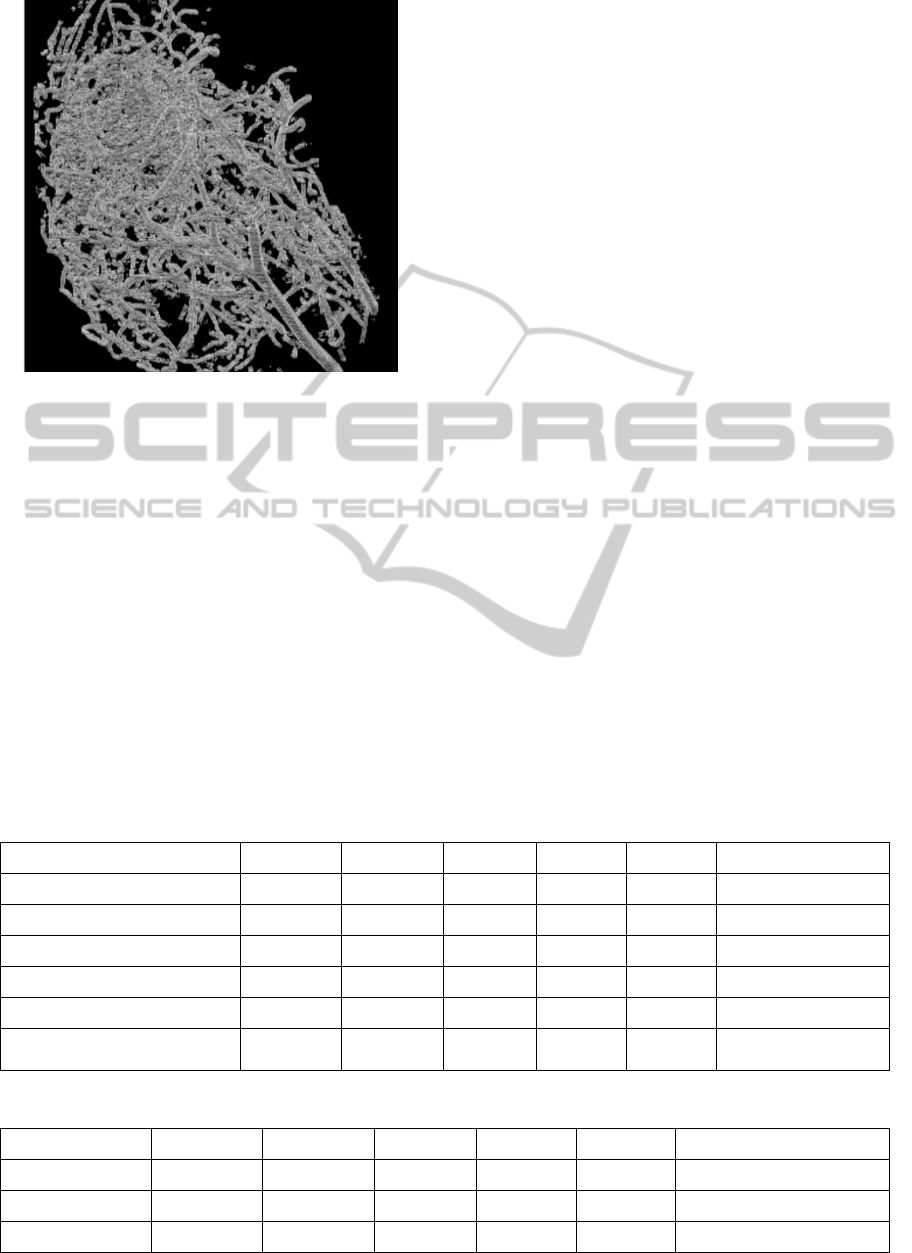
Figure 12: Result of WTMM in 3D.
3 COMPARISON AND ANALYSIS
Table 1 and 2 contain performance detail on each
database separately. Performance measures are
sensitivity, the percentage of correctly classified
blood-vessel pixels, obtained by TP/(TP+FN);
specificity, the percentage of correctly classified
non-blood-vessel pixels, obtained by TN/(FP+TN);
accuracy, how close the number of correctly
classified pixels is to the actual value, obtained by
(TP+TN)/(TP+FP+FN+TN) and precision, how
close the true positive and false positive are,
obtained by TP/(TP+FP); where T=TURE,
F=FALSE, P=POSITIVE and N=NEGATIVE.
3.1 2D
WTMM was the fastest. The speed of the vesselness
filter and LET were acceptable, but LET with Gabor
filter and all level set methods are slower due to
parameter selection for the Gabor filter. LET with
Gabor filter achieved the highest sensitivity
(89.83%). Both this method and our level set method
provided higher sensitivity as more vessels are
detected. WTMM
and LET produced low sensitivity
due to unconnected and missing vessels. Vesselness
filter has produced low sensitivity (62.64%) as user
selected scales and threshold values were susceptible
to errors. The best specificity obtained is by the
vesselness filter (98.74%), because it is robust to
image noise. While improved LET, level set
methods, and WTMM
are sensitive to image noise.
Vesselness filter produced the highest accuracy
(94.25%) whilst the results of LET and WTMM are
not good as a large number of vessels are missing or
disconnected. Vesselness filter achieved the highest
precision (87.64%).
3.2 3D
Implementation cost using vesselness filter and LET
remained acceptable. WTMM
took longer than 2
minutes. Both level set methods failed the
segmentation because it was computationally
expensive in 3D. Vesselness filter achieved the
highest sensitivity (86.26%) as more small vessels
were corrected detected than using LET. WTMM
failed the experiment because all vessels were
broader than the original vessels. All Specificity
Table 1: Performance Detail using 2D Retinal Vessel Image.
2D Sensitivity Specificity Accuracy Precision Run time Drawback
WTMM 0.4545 0.9518 0.8916 0.5648 0.27s Unconnected vessels
LET 0.7599 0.9621 0.9383 0.7282 2.15s Missing vessels
LET+Gabor Filter 0.8983 0.9435 0.9378 0.6955 16.15s Parameter selection
Phase Based Level Set 0.8567 0.9399 0.9299 0.6626 40.53s Early termination
PB Level Set+Matched Filter 0.8712 0.8610 0.8622 0.4631 25.46s Non-smooth vessels
Vesselness Filter 0.6264 0.9874 0.9425 0.8764 1.05s
Need user
interaction
Table 2: Performance Detail using 3D Rat Brain Vessel Image.
3D Sensitivity Specificity Accuracy Precision Run time Drawback
WTMM 0.4711 0.9895 0.9868 0.1889 255.35s Thick vessels
LET 0.4181 0.9989 0.9959 0.6668 33.81s Not scale-invariant
Vesselness Filter 0.8626 0.9985 0.9978 0.7468 74.67s Need user Interaction
ExperimentalComparisonofVasculatureSegmentationMethods
431

values were high as the amount of noise was very
little. The highest value obtained was by LET
(99.89%). Vesselness filtered image was much
similar to the expected result and it obtained the best
accuracy (99.78%) and precision (
74.68%).
4 CONCLUSIONS
We have reviewed and analysed a number of vessel
enhancement and segmentation algorithms using
both 2D and 3D image. Vesselness filter can be used
to detect vessels of varying scales. A potential
application of this method is to extract the brain
microvasculature and compare healthy and diseased
brains. LET has produced the highest sensitivity in
2D experiment but this method is recommended
only when the vessels are large and on a simple
background. Although WTMM
and level set method
failed the performance tests, they are capable of
detecting edges of large objects, such as brain
tumours. The main issue in this work is that the
performance test was not technically accurate due to
the poorly made ground truth and insufficient test
images so the 3D segmentation result has not been
100% validated. For further work we aim to produce
valid ground truth images for testing segmentation
algorithms. We will also continue to develop robust
wavelet filters and in combination with other
mathematical methods and metrics such as high-
order flows (Lim et al, 2013) non-Euclidean distance
functions (Pujadas et al, 2013) for handling
multiscale vessels and improving segmentation
speed and accuracy for microvascular analysis
(Ward et al, 2013).
ACKNOWLEDGEMENTS
We would like to thank S. Nakagawa and the late
Terry Parker in Biomedical Sciences; Lee Buttery
and Lisa White in Biomedical Sciences, University
of Nottingham, UK for providing the 3D images.
REFERENCES
Bedford, L., Hay, D., Devoy, A., Paine, S., Powe, D. G.,
Seth, R. & Mayer, R. J. (2008). Depletion of 26S
proteasomes in mouse brain neurons causes
neurodegeneration and Lewy-like inclusions
resembling human pale bodies. The Journal of
Neuroscience, 28(33), 8189-8198.
Chanwimaluang, T., & Fan, G. (2003, May). An efficient
blood vessel detection algorithm for retinal images
using local entropy thresholding. In Circuits and
Systems, 2003. ISCAS'03. Proceedings of the 2003
International Symposium on (Vol. 5, pp. V-21). IEEE.
Daugman, J. G. (1988). Complete discrete 2-D Gabor
transforms by neural networks for image analysis and
compression. Acoustics, Speech and Signal Processing,
IEEE Transactions on, 36(7), 1169-1179.
Ding, Y., Ward, W.O.C., Parker, T., Nakagawa, S.,
Buttery, L., White, L., Bai, L., (2013). Segmentation
of Mouse Brain Microvasculature from Micro-CT
Images Using Gabor filter and Local Entropy
Thresholding, International Symposium on Cerebral
Blood Flow, Metabolism and Function.
Frangi, A. F., Niessen, W. J., Vincken, K. L., & Viergever,
M. A. (1998). Multiscale vessel enhancement filtering.
In Medical Image Computing and Computer-Assisted
Interventation—MICCAI’98 (pp. 130-137). Springer
Berlin Heidelberg.
Fraz, M. M., Remagnino, P., Hoppe, A., Uyyanonvara, B.,
Rudnicka, A. R., Owen, C. G., & Barman, S. A.
(2012). Blood vessel segmentation methodologies in
retinal images–A survey. Computer methods and
programs in biomedicine.
Lathen, G., Jonasson, J., & Borga, M. (2008). Phase based
level set segmentation of blood vessels. In 19th IEEE
International Conference on Pattern Recognition.
Lim, P. L., Bagci, U., Bai, L. (2013). Introducing Wilmore
Flow into Level Set Segmentation of Spinal Vertebrae,
IEEE Transactions on Biomedical Engineering, Vol. 60,
No. 1.
Mallat, S., & Zhong, S. (1992). Characterization of signals
from multiscale edges. IEEE Transactions on pattern
analysis and machine intelligence, 14(7), 710-732.
Osher, S., & Sethian, J. A. (1988). Fronts propagating with
curvature-dependent speed: algorithms based on
Hamilton-Jacobi formulations. Journal of
computational physics, 79(1), 12-49.
Pal, N. R., & Pal, S. K. (1989). Entropic thresholding.
Signal processing, 16(2), 97-108.
Pająk, R. (2003). Use of two-dimensional matched filters
for estimating a length of blood vessels newly created
in angiogenesis process. Opto-Electronics Review,
11(3), 237-241.
Pujadas, E. R., & Bai, L. (2013). Non-Euclidean basis
function based level set segmentation with statistical
shape prior, IEEE EMBC2013, Osaka, Japan.
Sato, Y., Nakajima, S., Shiraga, N., Atsumi, H., Yoshida,
S., Koller, T., & Kikinis, R. (1998). Three-
dimensional multi-scale line filter for segmentation
and visualization of curvilinear structures in medical
images. Medical image analysis, 2(2), 143-168.
Staal, J., Abràmoff, M. D., Niemeijer, M., Viergever, M.
A., & van Ginneken, B. (2004). Ridge-based vessel
segmentation in color images of the retina. Medical
Imaging, IEEE Transactions on, 23(4), 501-509.
Rorden, C., Karnath, H. O., & Bonilha, L. (2007).
Improving lesion-symptom mapping. Journal of
cognitive neuroscience, 19(7), 1081-1088.
Ward, W., & Bai, L., (2013). Multifractal Analysis of
Microvasculature in Health and Diseases, IEEE
EMBC2013, Osaka, Japan.
VISAPP2014-InternationalConferenceonComputerVisionTheoryandApplications
432
