Polygonal Approximation of an Object Contour by Detecting Edge

Dominant Corners using Iterative Corner Suppression

Rabih Al Nachar

, Elie Inaty

, Patrick J. Bonnin

and Yasser Alayli

Department of Computer Engineering, University of Balamand, PO Box 100, Elkoura, Lebanon

Laboratoire d'Ingénierie des Systèmes de Versailles-LISV, 10-12 Av de l'Europe, 78140 Vélizy, France

Keywords: Straight Edges, Corners, Polygonal Approximation, Contour.

Abstract: A new algorithm to detect straight edge parts which form the contour of an object presented in an image is

discussed in this paper. This algorithm is very robust and can detect true straight edges even when their pix-

el's locations are not straight due to natural noise at the object borders. These straight edges are than used to

report and classify contour's corners according to their angle and their adjacent segments lengths. A new

technique for polygonal approximation is also presented to find the best set among these corners to con-

struct the polygon vertices that best describe the approximating contour. It starts by eliminating the corners,

one after the other using Iterative Corner Suppression (ICS) process. This in turn enables us to obtain the

smallest possible error in the approximation. Experimental results demonstrate the efficiency of this tech-

nique in comparison with recently proposed algorithms.

1 INTRODUCTION

The problem of straight edge detection can be de-

fined as follows: Given a binary image of edges ex-

tracted from a real image using an existing edge de-

tector based on Sobel, Prewitt, Kirsh or Canny algo-

rithms (Prewitt 1979, Sobel 1978, Kirsh 1971 and

Deriche 1987), find the parts of an edge that can be

classified as straight edges or segments of length

greater than a given threshold. The importance of

developing an algorithm that can detect these

straight edges remains a very important task in com-

puter vision and pattern recognition (Loncaric 1998).

In addition, straight edges are encountered a lot in

human made internal and external urban environ-

ments and objects. For example, Herman in (Herman,

Kanade and Kuroe 1984) presents an application for

an aerial robot to form and update of a 3D map of a

sequence of aerial scenes. The dedicated objects to

be detected in these images are the buildings. So he

identified them by their straight edges and their in-

tersection at the corners. Other applications are in-

door applications where a robot tries to build a map

of its environment and localize itself in it which is

called the SLAM problem. The target objects, used

for this purpose, are identified by their straight edges

like doors and walls intersection. In other applica-

tion, a combination of straight edges is used

(Bouchafa and Zavidovique 2006) to form specific

shapes like V-shape, W-shape and Z-shape. Each

shape is invariant under a specific image transfor-

mation. For this reason, it is used for image registra-

tion.

The most important objective of extracting

straight edges is their role in identifying corners that

are used as interest points in a lot of algorithms in

image processing. A corner (Nachar, Inaty, Bonnin

and Alayli 2012) can be defined as intersection of

non collinear straight edges with appropriate length.

From here, correct detection of straight edges will

lead to efficient corners detection.

After extracting the image corners based on

straight edges of a shape, we have developed a new

technique for "polygonal approximation" that con-

sists of selecting a number of well chosen corners to

construct the polygon that best approximates the

contour of that shape. Polygonal approximation is

widely used in object recognition (Ayache and

Faugeras 1986) because it smoothes the contour of

the objects in the images without loss of critical in-

formation. Related works to this algorithm are cited

in the next section.

The rest of the paper is organized as follows:

Section 2 presents some related works on polygonal

approximation. Section 3 describes the edge extrac-

tion and the chain code of every edge point. Section

247

Al Nachar R., Inaty E., J. Bonnin P. and Alayli Y..

Polygonal Approximation of an Object Contour by Detecting Edge Dominant Corners using Iterative Corner Suppression.

DOI: 10.5220/0004650602470256

In Proceedings of the 9th International Conference on Computer Vision Theory and Applications (VISAPP-2014), pages 247-256

ISBN: 978-989-758-003-1

 2014 SCITEPRESS (Science and Technology Publications, Lda.)

4 explains our proposed algorithm using polygonal

approximation. Experimental results are revealed in

Section 5. The conclusion is shown in Section 6.

2 RELATED WORKS

A large number of methods were proposed so far

(Dunham 1986). Pavlidis in (Pavlidis 1982) presents

an algorithm, known as split and merge technique. It

divides an edge into a set of segments that has each

one a maximal distance to the edge less than a given

threshold d as shown in Figure 1.

Figure 1: Polygonal Approximation.

The parameter used in this technique is the maximal

distance d

max

between the segment and the edge as

described in Figure 2. If d

max

is greater than the

threshold d, the segment [AB] is divided into two

segments; [AM] and [MB] where M is the edge

point corresponding to d

max

Figure 2: Segment division according to maximal distance.

Wall and Danielsson in (Wall and Danielsson 1984)

presented another algorithm that tries to find the

segment [AB] shown in Figure 2 by moving its end-

point B starting from the edge point A along the

edge until a certain criterion is no longer verified.

The criterion used here is the maximal area per unit

of length of the deviation between the edge and the

corresponding approximated segment that should be

less than a given threshold. Another technique for

obtaining a polygonal approximation of an object's

contour based on an updated Hough Transform is

presented in (Gupta, Chaudhury and Parthasarathy

1992). On the other hand, the method in (Mikheev ,

Vincent and Faber 2001) is dedicated for the pol-

yline representation of a scanned text or graphic

objects. Kolesnikov in (Kolesnikov 2008, 2009,

2011) focused on the approximation of a polygonal

edge or curve P of N vertices by another polygonal

edge Q with a minimal number of segments or verti-

ces M (M<N) while conserving a given criterion so

that the resulting error does not exceed a given

threshold. The error is the sum of the square distanc-

es of the N vertices of curve P relative to the curve

Q. Pinheiro in (Pinheiro 2010) searched for edge

points, called curvature extremes, that correspond to

a change in the direction of the curve (edge) using a

curvature function which form the polygon vertices.

These extremes are selected at different scale level

of the smoothed image. When the scale level in-

creases, the edge details become smoother so the

number of extremes will be reduced. Parverz and

Mahmoud in (Parvez and Mahmoud 2010) searched

for cut-points on the contour of the studied shape.

These points correspond to a deviation in the con-

tour direction. Then the algorithm tries to minimize

the number of detected cut-points until a terminating

condition is satisfied. The final approximated poly-

gon will have these cut points as extremes.

In (Carmona-Poyato, Madrid-Cuevas , Medi-

naCarnicer and Munoz-Salinas 2010), the authors

presented a technique based on detecting dominant

points on the contour and then iteratively suppress-

ing the redundant ones in order to obtain the best

approximated polygon with the minimal number of

segments. The algorithm of Masood in (Masood

2008) also detects first dominant points called break

points then starts to eliminate the ones with minimal

error value based on global measure. The optimal

result is not guaranteed even with the usage of an

optimization procedure. Finally, Marji and Siy in

(Marji and Siy 2004) presented a very similar tech-

nique to the one used in (Masood 2008) but it differs

by the measure of error of each dominant point.

Here, a dominant point is characterized especially by

its strength that means its non collinearity with re-

spect to its direct neighbors.

We have proposed in this paper an approach in-

spired by that presented in (Marji and Siy 2004 and

Masood 2008). We have searched for dominant cor-

ners that best approximate a given shape by a poly-

gon having these corners as vertices. The differences

between our work and their works are in the nature

and stability of the selected points and in the method

used to select these points among others. On the

other hand, the error measure used to eliminate or to

VISAPP2014-InternationalConferenceonComputerVisionTheoryandApplications

248

keep a corner is based on the Integral Square Error

between an edge part and the straight segment ap-

proximating it. So, it is similar to the criterion used

by Wall and Danielson (Wall and Danielsson 1984)

that relies on the area of the region included between

the edge part and its approximated segment rather

than only relying on the maximal distance like in the

method of Pavlidis (Pavlidis 1982).

3 EDGE EXTRACTION AND

CHAIN CODE

3.1 Edge Points Extraction

Given an original image, the extraction of edge

points is performed in several steps:

 Gradient computation: in norm (magnitude of the

edge) and direction (normal to the edge direction).

 Threshold on gradient norm, to extract initial edge

points.

 Thinning edge points to thin thick edges to one

pixel width.

 Prolongation of edge points to close open edges.

 Linking edge points to obtain edges (lists of

hooked edge points) from edge points.

Three possibilities to obtain gradient computation, in

norm and direction, which are:

1) Either Prewitt (Prewitt 1979) or Sobel Algorithm

(Sobel 1978), which consist in two steps :

 Compute the gradient projections on X and Y ax-

is, using two masks : Gx and Gy,

 then compute the norm and the direction using a

rectangular to polar transform,

2) Kirsh algorithm (Kirsch 1971), which obtains

directly the gradient in norm and direction, by

choosing the best approximation among the four

projections: horizontal, vertical, and two oblics

using four masks: Gx, Gy and G+45 and G-45.

3) Canny edge detector (Canny 1986 and Deriche

1987) using the first derivative of a Gaussian

function. The zero-crossing points are the edge

points.

3.2 Edge Chain Codes

Linking an edge pixel C consists of identifying the

direction of transfer from it to one of its eight neigh-

bors, who has the greatest gradient norm. This direc-

tion is one of the eight Freeman directions coded in

Figure 3.

Figure 3: Freeman Codes.

As a result, a linked edge can be viewed as a chain

of Freeman codes of length equal to the number of

linked edge pixels (edge length) minus one. As an

example, Figure 4 shows a particular edge of nine

pixels with its chain codes.

Figure 4: An edge with its chain codes.

4 POLYGONAL APPROXIMA-

TION

The main goal of this paper is to introduce an opera-

tor that is able to extract a polygon that best approx-

imate an object's contour. The operator's algorithm is

composed of three functions that work sequentially

as shown in Figure 5.

Figure 5: Algorithm's Block Diagram.

4.1 Straight Edge and Corner

Detectors

Our objective is to detect edge parts that can be con-

sidered straight using only their chain codes. Then,

the intersection edge points of every two non collin-

ear edge parts are detected as corners. To do that, we

must introduce the chain codes of straight edges.

4.1.1 Perfect Straight Edges

A perfect straight edge is an edge whose chain code

is composed of one code or two codes at maximum.

There are eight different straight edges correspond-

ing to a unique code among the eight Freeman codes.

For example, a perfect horizontal straight edge has a

chain code of only 0 or 4 and a perfect straight edge

PolygonalApproximationofanObjectContourbyDetectingEdgeDominantCornersusingIterativeCornerSuppression

249

along the first diagonal has a chain code of 1 or 5 as

shown in Figure 6.

In addition to these eight cases, a perfect straight

edge has a chain code composed of two codes: one

primary and the other secondary with a difference

equal to one between them. The classification of

these two codes is done according to their frequency

of occurrence in the edge's chain code. This is illus-

trated in Figure 7.

Figure 6: Straight Edges with unique code.

In Figure 7, five edges are considered starting

from one origin O. Edges1 and edge5 are those that

have a unique code 0 and 1 respectively, and their

slope are 0

and 45

. Edge3 is the one that have dou-

ble codes 0 and 1 of the same frequency of occur-

rence so its slope is 22.5

and it is the bisector of the

angle formed by edge1 and edge5. Edge2 is near to

edge1 and has also double codes 0 and 1 but with

different frequency of occurrence. Code 0 is primary

and code 1 is secondary. Same result can be seen in

edge4 that has code 1 as a primary and code 0 as

secondary.

Figure 7: Straight edges with double Freeman codes.

As a conclusion, we can say that the perfect straight

edges that have double codes are of two kinds. The

first kind of edges has double codes of same fre-

quency (edge3). It is equidistant between two

straight edges of unique code (edge1 and edge5).

The second kind of edges also has double codes but

of different frequency (edges2 and4) and it is also

between two straight edges of unique code corre-

sponding to the primary or secondary code. Here,

the nearest one's code forms the primary code. In

Figure 7, Edge1 is the nearest to Edge2, so the pri-

mary code for Edge2 is 0.

4.1.2 Algorithm Explanation and Real

Straight Edges

In real images, the chain code of a straight edge that

should be composed of one or two successive codes

has usually more than two codes. Our goal is to

identify which of them are the primary and second-

ary codes and reject the remaining codes. This prob-

lem is due to natural noise at the object borders.

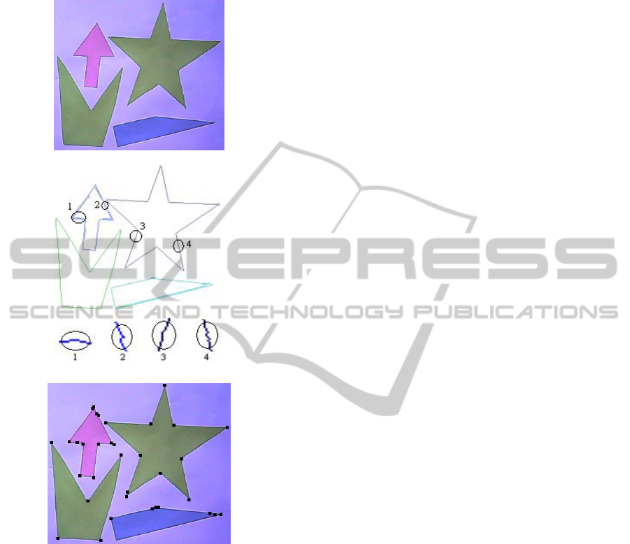
Real straight edges are shown in Figure 8 (a)

where some perturbations, circled in the image of

edges Figure 8 (b), are encountered along these edg-

es. The challenge is to build an intelligent algorithm

that can identify these perturbations and detect real

straight edges that meet at corner points as shown

with their angles in Figure 8 (c).

Our algorithm can be initiated at any edge point

E. The purpose is to test the existence of a real

straight edge with successive noisy pixels less than

m and of a length greater than a threshold d. The

idea behind the algorithm is to start testing an image

edge starting from its head to its tail. Consider the

first encountered edge direction as primary direction

and the next encountered edge direction as second-

ary edge direction. While moving the current pixel

to the tail, increment the frequency of primary or

secondary directions when the current pixel's direc-

tion corresponds to primary or secondary directions,

respectively. Or increment the frequency of noisy

pixels, if the current pixel's direction differs from

them. If the number of noisy pixels exceeds a given

threshold m, the edge test stops at the current pixel.

Now, if the edge length is greater than another

threshold d, the edge traversed so far is considered

as a straight edge.

Let us define the variables used in the algorithm:

- pdir: edge primary direction.

- pdirfreq: frequency of pdir.

- sdir: edge secondary direction.

- sdirfreq: frequency of sdir.

- cdir: current pixel direction.

- InfectedCount: number of noisy pixels en coun-

tered so far.

- el: edge length.

- SecondaryFound: a flag that is set when a second

VISAPP2014-InternationalConferenceonComputerVisionTheoryandApplications

250

ary direction is found.

- diff: absolute difference between cdir and pdir

(a)

(b)

(c)

Figure 8: (a) Real image, (b) image of edges, (c) detected

corners.

The algorithm details can be listed as follows:

 Record the first edge direction at E (Freeman

code) as pdir and initialize pdirfreq = 1. Initial-

ize InfectedCount = 0, el=1 and Second-

aryFound = false and proceed to the next linked

pixel.

 Iterate until the current pixel C reaches the tail

of the edge.

 Calculate diff .

 If (Not SecondaryFound):

 if (diff==1), record cdir as sdir, initialize

sdirfreq = 1 and put SecondaryFound = true.

 else if (cdir==pdir) than increment pdirfreq.

 else increment InfectedCount.

 Else

 If(diff>=2)or((diff==1)and(cdir!=sdir

))current pixel is a noisy pixel than in-

crement InfectedCount.

o if (InfectedCount>m): meaning

that we are reached the maximum

allowable noisy pixels: stopping

criterion=>Ends of straight edge

test:

 if(el>=d) than the current edge

is a real straight edge.

 else if (cdir==pdir) than increment

pdirfreq and set InfectedCount=0.

 else if (cdir ==sdir) than increment

sdirfreq.

 update pdir and sdir: pdir is the direc-

tion that has the maximum frequency

between (pdir, pdirfreq) and (sdir,

sdirfreq).

 el++.

A noisy pixel is an edge pixel, located on a real

straight edge, whose edge direction is different than

those of the corresponding perfect edge. From here,

the variable diff is introduced. Next, the search is for

the edge direction, if exists, that differs by one from

the primary direction pdir knowing that a perfect

straight edge can have a chain code composed at

maximum of two codes with difference equal to one.

The variable InfectedCount is incremented each time

a noisy pixel in encountered and it is cleared only if

the current edge pixel direction cdir is equal to pdir.

On the other hand, if cdir is equal to sdir, the varia-

ble InfectedCount should not be cleared. In Figure 9

(a), consider the example of a straight edge whose

pixels are in black. It is linked with pdir = 1 and sdir

= 2. At point A, the cdir is 3 so InfectedCount is

incremented. Next at point B, the cdir is 2 and it is

clear that the remaining edge in gray forms a differ-

ent straight edge. If we reset InfectedCount at B

when cdir = sdir = 2, the algorithm will not stop and

will consider both edges, in black and in gray, as one

straight edge which is incorrect. A final point should

be discussed which is the need to update pdir and

sdir. The logical reason for this case is that a straight

edge primary direction is not necessary the first en-

countered cdir as shown on the straight edge in Fig-

ure 9 (b). Initially pdir = 4 and sdir = 5. But after

traversing the remaining edge pixels, it is clear that

pdir should be 5 and sdir should be 4.

PolygonalApproximationofanObjectContourbyDetectingEdgeDominantCornersusingIterativeCornerSuppression

251

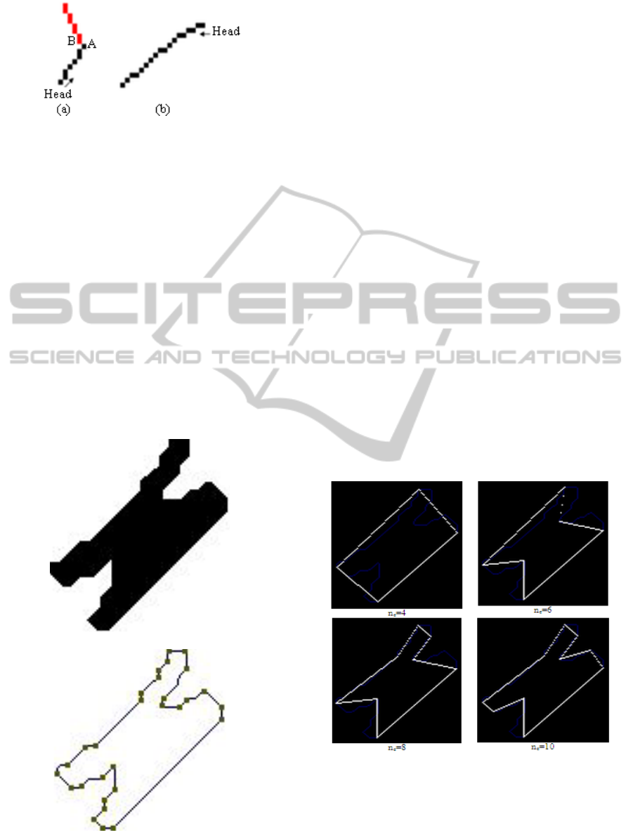
Figure 9: Two straight edges.

Finally, after the detection of straight edges the cor-

ner detection process starts by considering the inter-

section points of every two non collinear straight

edges as corners.

4.2 Polygonal Approximation using

Iterative Corner Suppression

In this section, we develop a novel technique based

on corner points called Iterative Corner Suppression

(ICS). Here, the corners, reported by the corner

detector, are characterized by the lengths of its two

sides (straight edges) and by its angle between its

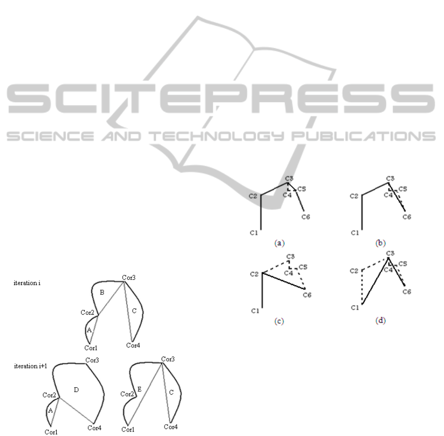
two sides. The corners for the chromosome shape in

Figure 10 are shown in the linked edge image in

Figure 10 (b) with their angle directions.

(a)

(b)

Figure 10: Detected corners for a chromosome shape: (a)

Chromosome shape, (b) Linked edge image.

The global algorithm starts with the straight edge

detector, detects the straight edges of every contour

in the image, and reports the intersection of every

two non collinear straight lines as corners. Then, the

polygonal approximation algorithm examines every

contour, selects from its corners the dominant ones

that form a polygon that best fit it.

Thus, the goal of our polygonal approximation

algorithm is to find the optimal polygon, approxi-

mating the contour of a given shape, given a re-

quired compression ratio CR:

 





⁄

(1)

where n is the number of shape's edge points and nc

is the number of selected corners called dominant

corners that form the polygon vertices. At a given

CR, the objective function is to minimize the global

integral square error (ISE) which is the sum of

squared distance of each contour's edge point to the

nearest approximated polygon segment. The ISE of

a polygon's segment corresponds to the area of the

region bounded between it and the corresponding

edge part. For a particular shape as in Figure 11,

since n is constant CR becomes a function of nc only.

Therfore, the problem is limited to obtain the mini-

mal possible ISE for a given number of dominant

corners nc. In general, the entry of the algorithm is

the parameter CR, nc will be calculated automatical-

ly for every contour.

Figure 11: Polygonal Approximation at various nc.

Figure 11 shows the approximated polygon of the

chromosome shape used in Figure 10 at various nc.

The global ISE decreases while nc increases.

Two parameters are used in the algorithm and

should be understood at the beginning. The first one

VISAPP2014-InternationalConferenceonComputerVisionTheoryandApplications

252

is the local ISE which is the ISE corresponding to a

given polygon's segment. The second one is the local

ISE variation "LISEV" due to the removal of a cor-

ner from the list of polygon's vertices. In Figure 12,

at iteration i+1, the LISEV due to the removal of

corner Cor3 has the same meaning as LISEV due to

the introduction of segment [Cor2Cor4]. The algo-

rithm can be summarized as follows:

 For a given contour of n edge points and m cor-

ners, select all the detected corners as polygon's

vertices following the linking order.

 The number of dominant corners nc = m.

 Iterate until the current CR = n/nc becomes

greater than or equal to a specified threshold.

 For each current corner "Corc" from the list

of selected corners:

 Find the previous and next selected corners

"Corp" and "Corn".

 Calculate the LISEV due to its removal:

LISEV

= new segment LISE – old segments

LISEs (see illustration in Figure 12).

 If any of the previously removed corner lo-

cated between "Corp" and "Corn" has a

greater LISE variation (LISEV

) than rese-

lect this corner, remove the current corner

"Corc" from the list of vertices and set the

final LISEV as LISEV

 Remove the corner that corresponds to the

minimal LISEV from the list of selected corner.

 Decrement nc by 1.

 Calculate the global ISE for the entire polygon

which is the sum of LISEs of introduced seg-

ments.

Figure 12: Corner Suppression.

Starting by considering all the corners as

polygon's vertices, the idea behind the ICS algorithm

is to decrease the number of vertices iteratively of

the approximated polygon. Here, the suppressed

corner (vertex) is the one that its suppression will

cause the minimal increase to the current global ISE

and this will ensure the selection of the optimal pol-

ygon at every iteration (at every value of nc). Con-

sider the case presented in Figure 12. We have four

selected corners at iteration i so there are three

polygon's segments with their corresponding LISE

represented by the areas A, B and C. The idea is to

calculate the LISEV caused by the removal of one of

the two corners Cor2 or Cor3, for example, at itera-

tion i+1. D is the area that represents the LISE of

Cor3 and E is the one that represents the ISE of Cor2.

The removal of Cor3 will add a new polygon's seg-

ment [Cor2Cor4] and eliminate two others

[Cor2Cor3] and [Cor3Cor4]. Therefore, we can

write

LISEV



DBC

(2)

Same procedure will apply for calculating the

LISEV caused by the removal of Cor2 with:

LISEV



E



AB



(3)

If LISEV

is smaller than LISEV

than Cor2 will be

removed otherwise Cor3 will be removed.

Figure 13: Corner Reselection.

While the corners are suppressed one after the other,

the LISEV of a corner that depends on the current

corner "Corc" and the directly selected neighboring

corners (previous one "Corp" and next one "Corn"),

may change since "Corp" or "Corn" may also

change. So we should always update and then check

the LISEV of even the suppressed corners to ensure

the optimality of the suppression at each iteration.

This can be illustrated using the list of corners

shown in Figure 13 where all the five corners are

selected initially. This is a tested case by the algo-

rithm where C4 (Figure 13 (a)), C5 (Figure 13 (b))

then C3 (Figure 13 (c)) are suppressed iteratively

PolygonalApproximationofanObjectContourbyDetectingEdgeDominantCornersusingIterativeCornerSuppression

253

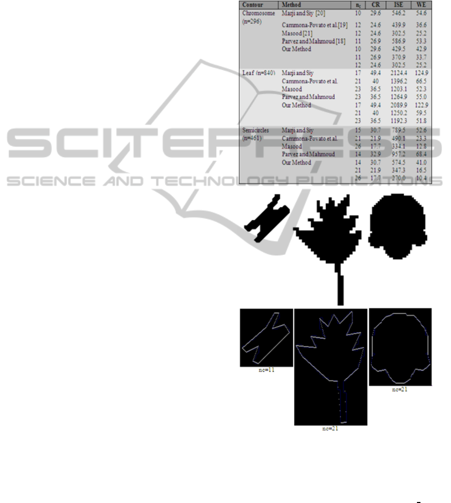
first and the remaining polygon has only C1, C2 and

C6 as vertices. Now if we calculate the LISEV of

removing C2 and that of removing C3, C4 and C5

taking C1 as "Corp" and C6 as "Corn", we find that

the LISEV of removing C3 is the greatest one. So

we should suppress C2 and reselect C3 (Figure 13

(d)). Then, the LISEV resulting from adding [C1C6]

is that of removing C3 and it will be compared with

the LISEV of removing the remaining selected cor-

ners existing on the whole contour to deselect the

corner with the minimal one.

5 EXPERIMENTAL RESULTS

Our proposed algorithm is tested on three different

shapes shown in Figure 14: (a) Chromosome, (b)

Leaf and (c) semicircles (The and Chin 1989). The

results obtained are compared to those presented in

various papers (Parvez and Mahmoud 2010, Carmo-

na-Poyato, Madrid-Cuevas, MedinaCarnicer and

Munoz-Salinas 2010, Marji and Siy 2004 and

Masood 2008).

Other than the ISE, a new parameter is intro-

duced for the comparison: the weighted sum of

square error WE given by

 







(4)

Since our algorithm requires a colored or grey image

as an input not only a digital image or edge image

while the others are tested directly on a digital image,

we need a unique platform for comparison. From

here, we have selected manually on the edge image

derived by our algorithm the vertices of the polygon

reported by each method in (Parvez and Mahmoud

2010, Carmona-Poyato, Madrid-Cuevas, Medi-

naCarnicer and Munoz-Salinas 2010, Marji and Siy

2004 and Masood 2008), then calculate the corre-

sponding ISE and show the results in Table 1.

From Table 1, it can be seen clearly that our algo-

rithm has better ISE and WE compared to others.

This is due to three main reasons. The first one is the

excellent location of the corners due to the efficient

straight edge detector. So, the optimal polygon is the

one whose vertices are selected among these corners.

The second one is the efficient technique to select

the best corners as polygon vertices that will lead to

the minimal error (ISE) at a specific nc. The third

one is the update of the LISE, at each iteration, even

for previously suppressed corners. This feedback

will ensure that, when eliminating a corner or select-

ing a new segment, the maximal LISE is set for this

segment. This fact will show the real LISEV caused

by selecting this segment and as a result will ensure

the selection of the segment with the real minimal

LISEV.

Table 1: Comparative Results for the Chromosome, Leaf

and semicircle shapes.

(a) (b) (c)

Figure 14: Tested Shapes and their polygonal approxima-

tions at a particular nc.

For a real image that contains more than one shape

or contour, nc cannot be fixed and considered as an

input for the algorithm since existing contours may-

be best approximated by polygons of different num-

ber of vertices. In other words, nc cannot be fixed

for all contours. Here, CR or WE plays the big role

VISAPP2014-InternationalConferenceonComputerVisionTheoryandApplications

254

and must be used both or at least one of them as in-

puts. By specifying a threshold for the WE parameter

used as an input, the role of a polygonal approxima-

tion algorithm becomes to find the greatest nc per

contour that corresponds to the greatest WE less than

the specified threshold. Here the CR is an output. On

the other hand, by specifying a threshold for CR

used as an input, the goal still to find the greatest nc

per contour, that corresponds to the minimal CR

greater than the threshold. In this case, WE is an

output. So the choice of selecting which parameter

or maybe both depends on the specific application.

Finally, Figure 14 shows the polygons approxi-

mating the tested shapes at a given nc. It can be seen

clearly that the results are very precise.

Finally, we suggest an application based on DCs

which is shape recognition of 2D objects dedicated

for a robot embedded with a vision system where

our polygonal approximation's algorithm is imple-

mented. The goal is to present first a 2D shape to the

robot and then it tries automatically to locate it in a

simple scene.

To simulate this experiment, we present two im-

ages to the algorithm; the first one is a training im-

age, shown in Figure 15, containing only the desired

shape and the second one is a test image containing

a scene of multiple shapes as shown in Figure 16 (a).

For the training image, the algorithm detects the

DCs located on the shape's contour. For the test one,

it detects and groups the DCs per contour represent-

ing each shape. After that the matching procedure

starts by comparing every test group of DCs with the

trained DCs using the DC angle and ratio of the

lengths of their sides as matching parameters.

Figure 15: Training image.

This matching criterion remains feasible when the

image transformation that relates the two images is a

translation-rotation, similarity or conditioned affinity.

In general, an affine transformation preserves ratio

but does not preserve angles (Hartley and Zisserman,

2003) so the matching criterion does not hold for

this type of transformation only if the camera plane

and the shape plane are parallel (Hartley and Zis-

serman 2003); in this case, the angles are nearly pre-

served. This is the conditioned affinity.

The result of matching is shown in Figure 16 (b)

where the DCs are shown only on the matched

shape's contour which is the star shape.

(a)

(b)

Figure 16: (a) Test image. (b) Corresponding Image of

contours with DCs shown on matched contour.

6 CONCLUSIONS

In this paper, a new polygonal approximation tech-

nique is proposed. It is composed of two procedures.

The first is called "Straight Edges Detector" which

examines all the contours existing in the input image

and detects the edge parts that can be considered as

straight edges. These straight edges are straight lines

that exist frequently at the borders of various objects

in real scenes especially human made environments

like buildings, cars, doors… The importance of de-

tecting these straight edges remains in their role of

detecting edge corner points. The intersection of two

non collinear straight edges of appropriate length

(greater than a threshold) is reported as a corner.

The second part of our work is a polygonal ap-

proximation algorithm that takes the detected cor-

ners as an entry. By fixing an entry parameter like

PolygonalApproximationofanObjectContourbyDetectingEdgeDominantCornersusingIterativeCornerSuppression

255

Compression ratio CR or weighted sum error WE,

the algorithm starts, per contour, by removing itera-

tively the corners that introduce the minimal possi-

ble ISEV to the global ISE measure until reaching

the stopping criterion. At the end, the remained cor-

ners form the vertices of the polygon that can best

approximate the current contour.

The experimental results have shown good re-

sults in comparison with other existing methods. In

our opinion, this is due to the efficient straight edge

detector that explores all the contour corners effi-

ciently and then to the iterative polygonal approxi-

mation algorithm that removes, at each iteration, the

corner with the smallest LISEV and at the same time

updates and reexamines the LISEV of already re-

moved corners. This way, we can ensure that the

remained corners form the polygon that best fit their

contour.

Finally, as a future work, we suggest an image

registration application that can benefit from detect-

ed straight edges and corners. These image features

can be combined together in a certain number to

form specific shapes or primitives that can have in-

variant measures versus different image transfor-

mation.

REFERENCES

Loncaric, S., 1998. A survey of shape analysis techniques,

Pattern Recognition, vol.31.

Herman M., Kanade T. and Kuroe S., 1984. Incremental

Acquisition of a Three-Dimensional Scene Model from

Images, IEEE Transactions on Pattern Analysis and

Machine Intelligence, Vol. Pami-6, No. 3.

Bouchafa S. and Zavidovique B., 2006. Efficient cumula-

tive matching for image registration. Image and Vi-

sion computing, Vol. 24.

Ayache N. and Faugeras O., 1986. A new approach for the

recognition and positioning of two dimensional ob-

jects, IEEE Transaction on Pattern Analysis and Ma-

chine Intelligence, vol.8.

Nachar R., Inaty E., Bonnin P. and Alayli Y., 2012. A

Robust Edge Based Corner Detector, Submitted for

possible publication in Autonomous Robots Springer,

September 2013, under review.

Dunham J.,1986. Optimum Uniform Piecewise Linear

Approximation of Planar Curves, IEEE Trans on Pat-

tern Analysis and Machine Intelligence vol PAMI 8

n°1, pp 67-75.

Pavlidis T., 1982. Algorithms for Graphics and Image

Processing, Springer Verlag.

Wall K. and Danielsson P., 1984. A fast sequential method

for polygonal approximation of digitized curves,

Computer Vision Graphics and Image Processing, vol

28, pp 220-227.

Gupta A., Chaudhury S. and Parthasarathy G., 1992. A

Hough Transform Based Approach to Polyline Ap-

proximation of Object Boundaries, Proceedings. 11th

IAPR International Conference on Pattern Recognition.

Vol.III. Conference C: Image, Speech and Signal

Analysis.

Mikheev A., Vincent L. and Faber V., 2001. High-Quality

Polygonal Contour Approximation Based on Relaxa-

tion, Pr ceedings Sixth International Conference on

Document Analysis and Recognition.

Prewitt J., 1979. Object enhacement and extraction, Pic-

ture processing & psychopictorics, BS Lip-

kin&A.Rosenfelded, Academic Press, New York USA.

Sobel, 1978. Neighbourhood coding of binary images for

fast contour following and general binary array pro-

cessing, Computer Graphics & Image Processing USA,

vol 8 pp 127-135.

Kirsch R., 1971. Computer determination of the constitu-

ent structure of biological images, Computers and Bi-

omedical Research 4.

Kolesnikov A., 2008. Fast Algorithm for ISE-Bounded

Polygonal Approximation, 15th IEEE International

Conference on Image Processing.

Kolesnikov A., 2009. Minimum Description Length Ap-

proximation of Digital Curves, 16th IEEE Internation-

al Conference on Image Processing.

Kolesnikov A., 2011. Nonparametric Polygonal and Mul-

timodel Approximation of Digital Curves with Rate-

Distortion Curve Modeling, 18th IEEE International

Conference on Image Processing.

Pinheiro A., 2010. Piecewise Approximation of Contours

Through Scale-Space Selection of Dominant Points

IEEE Transaction on Image Processing, Vol. 19, No. 6.

Parvez M. T. and Mahmoud S. A., 2010. Polygonal Ap-

proximation Of Planar Curves Using Triangular Sup-

pression, 10th International Conference on Infor-

mation Science, Signal Processing and their Applica-

tions.

Carmona-Poyato A., Madrid-Cuevas F.I., MedinaCarnicer

R. and Munoz-Salinas R., 2010. Polygonal approxi-

mation of digital planar curves through break point

suppression, Pattern Recognition, 43( 1), pp. 14-25.

Marji M. and Siy P., 2004. Polygonal representation of

digital planar curves through dominant point detec-

tion – a nonparametric algorithm, Pattern Recognition

37, pp. 2113- 2130.

Masood A., 2008. Optimized polygonal approximation by

dominant point deletion, Pattern Recognition 4 1, pp.

227- 239.

The C. H. and Chin R.T., 1989. On the detection of domi-

nant points on digital curves, IEEE Transactions of

Pattern Analysis and Machine Intelligence 11, pp.

859-872.

Canny J., 1986. A computational approach to edge detec-

tion, IEEE Transactions of Pattern Analysis and Ma-

chine Intelligence., vol. PAMI-8, pp. 679–698.

Deriche R., 1987. Optimal Edge detection using recursive

filtering, Int journal on Computer Vision.

Hartley R. and Zisserman A., 2003. Multiple View Geome-

try in Computer Vision, Cambridge university press,

Edition.

VISAPP2014-InternationalConferenceonComputerVisionTheoryandApplications

256