
Image Registration based on Edge Dominant Corners
Rabih Al Nachar
1
, Elie Inaty
1
, Patrick J Bonnin
2
and Yasser Alayli
2
1
Department of Computer Engineering, University of Balamand, PO Box 100, Elkoura, Lebanon
2
Laboratoire d'Ingénierie des Systèmes de Versailles-LISV, 10-12 Av de l'Europe, 78140 Vélizy, France
Keywords: Image Edges, Dominant Corners, Affine Transformation, Polygonal Approximation, Primitive.
Abstract: This paper presents a new algorithm for image registration working on an image sequence using dominant
corners located on the image's edges under the assumption that the deformation between the successive
images can be modeled by an affine transformation. To guarantee this assumption, the time interval between
acquired images should be small like the time interval in a video sequence. In the edge image, dominant
corners are extracted per linked contour and form a polygon that best approximates the current linked
contour. The number of these dominant corners per contour is derived automatically given an approximation
error. These dominant corners are shown to be very repeatable under affinity transformation. Then, a
Primitive is constructed by four dominant corners. The invariant measure that characterizes each primitive is
the ratio of areas of two triangles constructed by two triplets selected from these four corners.
1 INTRODUCTION
Image registration (Zitova and Flusser, 2003) is the
process that determines the geometric model or
transformation that aligns the points in two images
of the same scene taken at different viewpoints,
different times, or even different camera types.
It is used in different fields like image matching
(Almehio and Bouchafa, 2010), stereovision
(Gouiffes, Lertchuwongsa and Zavidovique, 2011),
image mosaicking and animation (Wong, Kovesi
and Datta, 2007 and Zhi-guo, Ming-Jia and Yu-
qing, 2012), motion analysis (Bouchafa and
Zavidovique, 2006) and especially medical imaging
(Maurer and Fitzpatrick, 1993). The new image
registration algorithm presented in this paper is
targeting mainly motion analysis where the
deformation between the source image and the
target one can be modeled by an affine
transformation.
In recent years, many approaches have been
developed in this area, leading to a great evolution
of registration techniques (Zitova and Flusser,
2003). Those techniques can be classified in general
as spatial or frequency domain techniques. Spatial
methods rely directly on image intensities or image
features like edges (Wenchang, Jianshe, Xiaofei and
Lin, 2010 and Zhi-guo, Ming-Jia and Yu-qing,
2012), contours (Kumar, Arya, Rishiwal, and
Joglekar, 2006 and Li, Manjunath and Mitra, 1995),
regions (Chum and Matas, 2006), interest points
(Lin, Du, Zhao, Zhang and Sun, 2010) and lines
(Almahio and Bouchafa, 2010). While frequency
methods apply phase correlation between the pair of
images to extract the transformation model
(Wolberg and Zokai, 2000).
An application for the presented algorithm is
also camera stabilization in video mode for
smoothing the movement by reducing the effect of
camera in motion. The video images acquired have
a small time interval between them so the
deformation can be well modeled by an affine
transformation.
This paper is organized as follows: Section 2,
explains how an existing polygonal approximation
algorithm extracts dominant corners. In Section 3
we describe the first proposed process which is the
automatic selection of these corners. We present the
primitive construction procedure and its invariant
measure and explain the concept of voting scheme
in section 4. Section 5 shows some experimental
results on synthetic and real images. Finally, a
conclusion presents a summary of the work.
433
Al Nachar R., Inaty E., J. Bonnin P. and Alayli Y..
Image Registration based on Edge Dominant Corners.
DOI: 10.5220/0004650704330440
In Proceedings of the 9th International Conference on Computer Vision Theory and Applications (VISAPP-2014), pages 433-440
ISBN: 978-989-758-003-1
Copyright
c
2014 SCITEPRESS (Science and Technology Publications, Lda.)

2 AN OVERVIEW ON
POLYGONAL
APPROXIMATION AND
DOMINANT CORNERS
Edges are one of the most important features in the
image domain that have great immunity against
contrast variation. On these edges, corners (Nachar,
Inaty, Bonnin and Alayli, 2012 and 2013), which
are the intersections of non collinear straight edges,
are extracted. Among these corners dominant
corners (DCs) are selected. These DCs construct the
vertices of the polygon approximating a linked edge
or contour. Next, we will summarize the process of
corners elimination to have only DCs. More details
can be found in (Nachar, Inaty, Bonnin and Alayli,
2013)
2.1 Integral Square Error of a
Segment
Each segment joining two corners is characterized
by a measure called Integral Square Error (ISE)
between the portion of the edge limited by those
two corners and the segment itself (Carmona-
Poyato, Madrid-Cuevas, Medina Carnicer and
Munoz-Salinas, 2010).
2.2 Iterative Elimination of Corners
The process of corners elimination is an iterative
process. Initially, each corner C is represented by
the ISE of the segment joining its two direct
neighbors [CpCn] as described in Figure 1. The
term Global ISE denoted by GISE is the sum of all
segments ISEs.
Figure 1: Corner Elimination.
Consider the edge part shown in Figure 1.
Figure 1 (a) show an edge part in bold, three corners
and the two segments of a polygon joining them.
Figure 1 (b) shows the resulting segment [CpCn]
due to the removal of corner C. The elimination of a
corner is based on a measure called "Cost of
Removal" denoted by CR which is the error induced
to the GISE if the current corner is removed.
Mathematically, if C is the current corner, its CR is
(1)
CR
c
represent the area of the triangle
.
Iteratively, the corner C with the smallest CR is
removed first, its CR is added to GISE and the CR
of the direct neighbors is updated since Cn becomes
a direct neighbor for Cp instead of C and vise versa.
Finally, these non eliminated corners are the
DCs and form the vertices of the polygon
approximating the edge (Nachar, Inaty, Bonnin and
Alayli, 2013).
3 PROPOSITION ONE:
AUTOMATIC SELECTION OF
DOMINANT CORNERS AND
STOPPING CRITERION
The basic feature that should be added to the
algorithm presented in (Nachar, Inaty, Bonnin and
Alayli, 2013) in order to be used in an application
like image registration is the automatic selection of
dominant corners. The goal is to select only the
corresponding DCs on every couple of
corresponding contours in both images. Assume
that two images are taken of the same scene but at
different viewpoints, non corresponding edges
could appear. Even corresponding edges in the two
images may have different number of corners.
Therefore, we cannot rely on a compression factor
as a stopping criterion because it will lead to a lot of
non corresponding corners. On the other hand, even
corresponding corners may have different ISE
values if the scaling factor relating the two images
is relatively high.
Figure 2: Grouping four consecutive DCs into one
primitive.
VISAPP2014-InternationalConferenceonComputerVisionTheoryandApplications
434

As mentioned in Section 2, the basic measure
according to it a corner could be removed is the CR
that will be added iteratively to the GISE. From one
side, this GISE is equal to the sum of ISEs of
segments constructed by non eliminated corners
where each ISE is equivalent to the area limited by
the corresponding segment and edge part. So, GISE
is a sum of areas which is an area. On the other
hand, the affine transformation has the ratio of areas
an invariant parameter (Hartley and Zisserman,
2003). So taking the ratio of the current GISE with
respect to the initial one is a good measure that can
be used as a stopping criterion. While eliminating
the corners one after the other, GISE will increase.
Thus, we can stop the elimination automatically by
setting a fixed threshold r. This way, even when the
scaling parameter between the two images is
considerable, we can still obtain only corresponding
DCs in both images.
Affine transformation has the ratio of areas as an
invariant parameter, thus the ratio of CRs is
preserved under affine transformation. Therefore,
we can state that any two CRs (CR1 > CR2)
corresponding to two corners on the same contour,
will remain in the same order under an affine
transformation. So, the order of CRs is invariant
with respect to an affine transformation. Therefore,
we expect that only corresponding DCs will show
up in an image and the transformed one since the
elimination of a corner is based on its CR value
compared to others CRs.
4 PROPOSITION TWO:
GROUPING DCS INTO
PRIMITIVES AND VOTING
SCHEME:
4.1 Primitive Construction
Based on high reoccurrence of DCs, a primitive is
formed by grouping four consecutive DCs. The
average of the four corners ISEs is set as the
primitive ISE. Here, primitives are classified
according to their ISE. The strongest primitives are
those who have the highest ISEs. The vote of each
primitive will be biased by its ISE since strong
primitives are formed by DCs of high ISEs. This
means that the corners are of high repeatability or
high probability of occurrence in both images.
In Figure 2, a polygon of fifteen DCs as vertices
approximating the contour of a leaf image is shown.
The four circled DCs are grouped into one
primitive. Two triangles DC1DC2DC3
and
DC2DC3DC4
are considered. The ratio of their area
R will be used for matching with other primitives in
the second transformed image.
Consider now two images related by an affinity.
The primitives are formed in both images and each
primitive is characterized by its two parameters R
and ISE. We adopt a group voting scheme based on
Hough transform (Zhongke, Xiaohui and Lenan,
2003) for the six unknown parameters of the affine
transformation. The idea behind the Hough
transform is to accumulate, in a space of
representative parameters, the information that
assures the presence of a certain shape or model. In
our case, the desired model to find is an affine
model that has six unknowns. So, our Hough space
has six parameters and each matched couple of
primitives from the two images will increase by one
the accumulator of the corresponding point in this
space. Three points are enough to calculate these
parameters. Each primitive will vote for a set of six
parameters and the set that gets the highest votes
will be selected. Let DC
1
(x
1
,y
1
), DC
2
(x
2
,y
2
),
DC
3
(x
3
,y
3
) and DC
4
(x
4
,y
4
) be the DCs constructing
a primitive in the first image and DC'
1
(x'
1
,y'
1
),
DC'
2
(x'
2
,y'
2
), DC'
3
(x'
3
,y'
3
) and DC'
4
(x'
4
,y'
4
) be the
DCs constructing the corresponding primitive in the
second image. The affine transformation presented
in (1) can be rewritten as,
′
′
′
1
1
1
′.
(2)
′
′
′
1
1
1
′.′
(3)
The affine parameters presented in vectors h and h'
are calculated in (4) and (5), respectively:
.
(4)
.
(5)
4.2 Corresponding Primitives Refining
Using only the ratio R to match two primitives will
lead to a lot of false positive matches. This means
that two non corresponding primitives that have
similar ratio of areas are considered by the
algorithm as corresponding. To minimize or even
eliminate these false positives, we propose to use
the corners directions. These directions are the
directions of the two meeting straight edges coded
in Freeman code (0,4 for horizontal right-left, 2,6
for vertical up-down, 1,5 for first diagonal and 3,7
ImageRegistrationbasedonEdgeDominantCorners
435

for second diagonal (Freeman and Davis 1977)). We
show experimentally that the detected corners are
very repeatable against affine transformation. Also
they conserve their angle directions.
Figure 3: Two corresponding corners.
Figure 3 shows two corresponding corners C1
and C2 rotated by 180
o
one with respect to the
other. It is clear that the difference between dir1 of
both corners is equal to that between dir2. This
difference reflects the amount of rotation between
the two corners. Our proposition for correspondence
and voting is stated as follows:
For every couple of primitives P
1
and P
2
having similar ratio R.
If the difference between the directions of the
four corresponding corners in both primitives
is the same:
Form four triplets of three points in each
primitive. For example in P1: S
1
=
{DC
1
, DC
2
, DC
3
}, S
2
= {DC
1
, DC
2
,
DC
4
}, S
3
= {DC
1
, DC
3
, DC
4
} S
4
= {DC
2
,
DC
3
, DC
4
}.
Use the four sets in P
1
with those
corresponding sets in P
2
to calculate
four affine models.
Calculate the mean model AM
m
.
If the difference between the models is
relatively small, we report that P
1
and
P
2
are corresponding and at the same
time they give their vote for AM
m
.
Else, select a new couple of primitives.
Using this method, we involve the four points in the
parameters calculation. Here if two primitives are
really corresponding, the included corners should
have same directions difference and also the four
formed models should be very close. When the
number of votes is not relatively high, we can form
an additional set of primitives and thus an
additional number of voters. In this set, a corner is
grouped with its three nearest neighboring DCs to
form a primitive. This way of grouping is also
invariant under various transformations. The overall
algorithm is fully presented in Figure 4.
Figure 4: Proposed algorithm.
VISAPP2014-InternationalConferenceonComputerVisionTheoryandApplications
436
5 EXPERIMENTAL RESULTS
The experimental results are shown using synthetic
and real images. First, a source synthetic image is
used and the target image is generated using a well
known affine transformation. Thus, the six affine
parameters are known a priori. The first results will
show the accuracy of the algorithm by showing the
relative error between the generated affine model by
our algorithm and the given one. The second part
will show the repeatability of DCs under various
deformations between the source and target images
caused by affine transformation. In the third part,
synthetic images presented in (Almehio, 2012) are
used to compare their results with ours. Given the
affine model, the mapping between DCs in the
source image and those in the target is known and it
is used to show their repeatability.
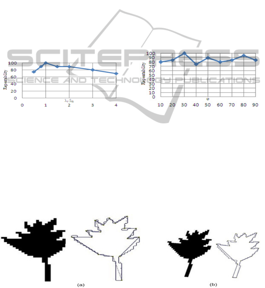
Figure 6: Repeatability of DCs versus scaling factor λ
1
/λ
2
(θ = 10
o
, φ = 15
o
and λ
2
= 1).
Figure 5 shows a source leaf image and its target
generated using an affine model with the following
values: a
11
= 0.8800, a
12
= 0.1907, a
21
= -0.1008, a
22
= 0.7728 (corresponding to θ = 10
o
, φ = 15
o
, λ
1
=
1.1 and λ
2
= 1.3 presented in section 2), t
x
= -150, t
y
= 15. Setting the threshold r (ratio of current GISE
and intial GISE used as a stopping criterion as
described in section 4) to be r=5, the number of
DCs extracted in the source image shown in Figure
5 (a) is 16 out of 98 corners while their number in
the target image shown in Figure 5 (b) is 17 out of
122 among them 15 DCs are corresponding ones.
In Figure 6, the repeatability of DCs versus the
scaling factor λ
1
/λ
2
is evaluated. The minimal value
of this repeatability is 70% at scale ratio of four
which is considered high when dealing with the
suggested application of video image sequence with
small interval time. Figure 7 shows the repeatability
of DCs versus scaling angle φ. It is clear that the
worst repeatability is 75% which is also very good
and will lead to a high repeatability of the formed
primitives. Figure 8 presents the repeatability versus
the rotation angle θ between the source and the
target images. Also, the worst repeatability is 85%
which means that the rotation angle θ has the least
influence on the repeatability value. In these results,
we have selected the stopping criterion as the
remaining number of DCs. It was chosen equal to
20DCs.
Figure 7: Repeatability of DCs versus scaling angle φ (θ
= 10
o
, λ
1
=1.3 and λ
2
= 0.8).
We can even obtain higher repeatability if we
select for example 80% of these DCs that
correspond to the highest ISEs. In Figure 7, it is
shown that for the given values of the affine
parameters (φ = 10
o
, λ
1
=1.3, λ
2
= 0.8 and θ=90
o
)
the repeatability of DCs is 85% (17 corresponding
DCs out of 20). If we select only 80% of these DCs,
the repeatability becomes 93.75% (15
corresponding DCs out of 16).
Now we will show the relative error between the
real affine model relating two synthetic images and
the estimated model by our algorithm. These
Figure 5: Polygonal Approximation and DCs of a source and target leaf images.
ImageRegistrationbasedonEdgeDominantCorners
437
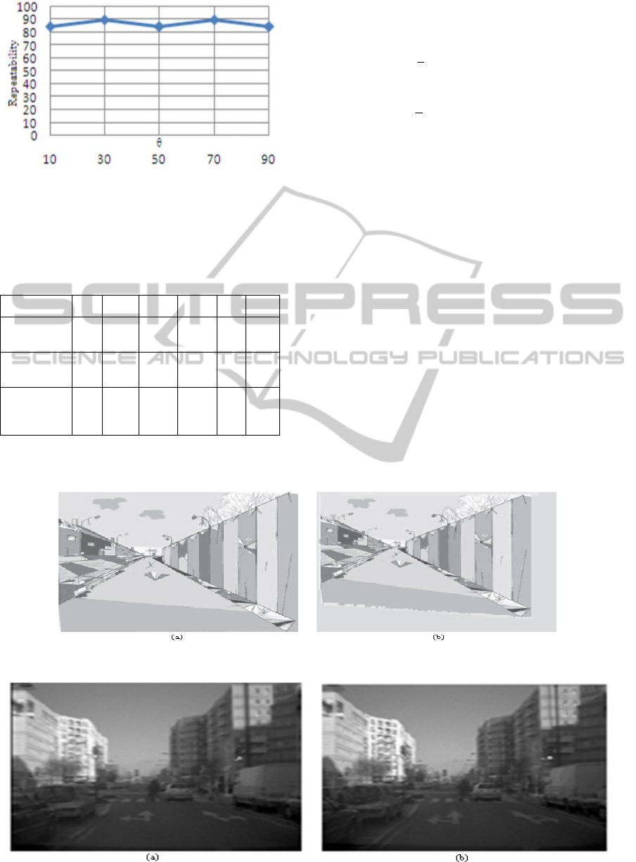
Figure 8: Repeatability of DCs versus rotation angle θ (φ
= 10
o
, λ
1
=1.3 and λ
2
= 0.8).
images (Almehio, 2012) are shown in Figure 8 and
the results are reported in Table 1.
Table 1: Estimated affine models.
a
11
a
12
a
21
a
22
t
x
t
y
Real Model
M
0.9 0 0.05 0.85 0 0
Our Model
M'
0.91 -0.04 -0.04 0.81 2 4
Model M'' in
(Almehio
2012)
0.88 0.008 0.05 0.85 -0.1 -7.7
To compare the results presented in Table 1, the
mean square errors MSE
o
between our model and
the real one and MSE
A
between Almehio model and
the real one are derived in (6) and (7).
1
6
′
3.335
(6)
1
6
′′
9.883
(7)
Figure 10 shows two real images taken from a video
sequence in (Almehio and Bouchafa, 2010). Two
matched primitives are shown in Figure 9 and the
image of difference between the source and target
images is revealed in Figure 11. In this image, each
pixel's intensity is obtained by taking the absolute
difference of corresponding pixels intensities in
both images. Thus darker pixels represent higher
difference between the compared intensities. Also,
the alignment between the two images is shown in
Figure 11. Let us concentrate on the arrow shape
circled in both images source and target of Figure
11. We see, in Figure 12, that part of this shape is
dark and part is bright. The dark part correspond to
a big difference between the two arrow shapes in
the source and target images and that is normal due
to the difference in the 3D position of the two
shapes. Thus, aligning these two shapes will make
the intersection part bright and the other part dark in
the image of difference. The same discussion can be
made on every corresponding part in both images.
Figure 9: Synthetic images (Almehio, 2012). (a) Source image. (b) Target image.
Figure 10: Two tested real images of a common scene (Almehio and Bouchafa, 2010).
VISAPP2014-InternationalConferenceonComputerVisionTheoryandApplications
438
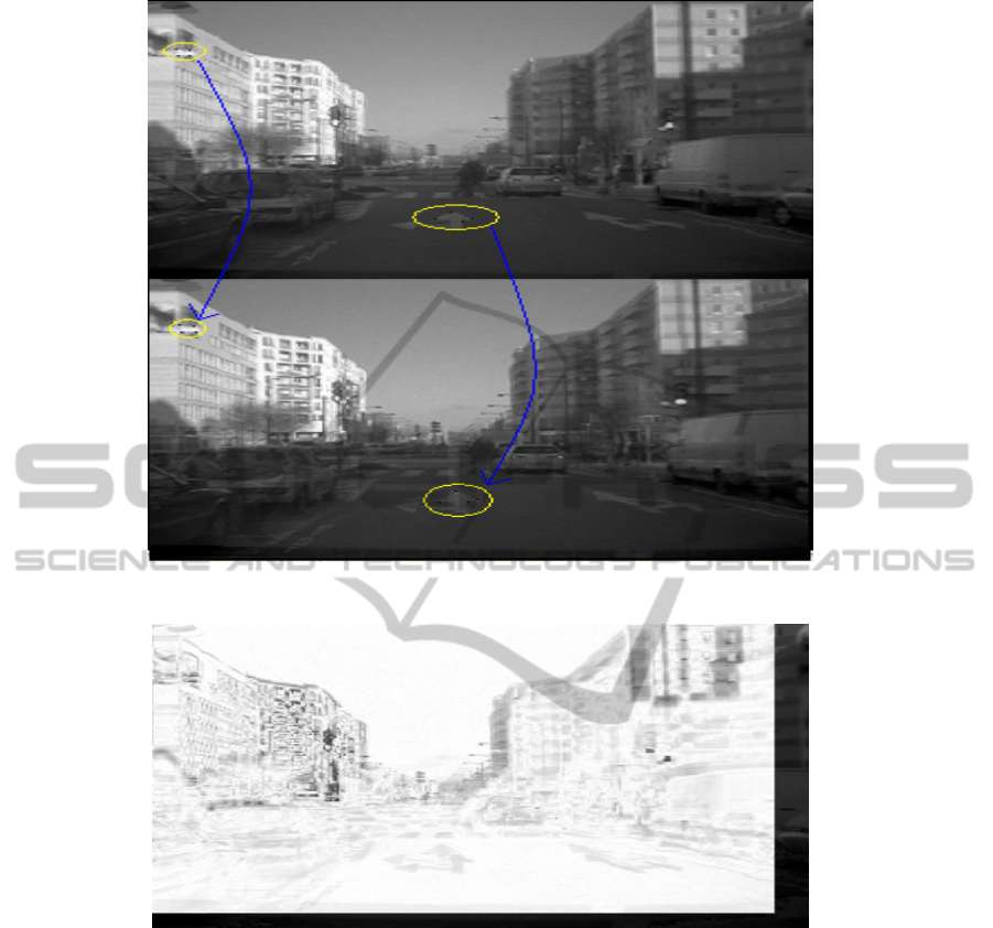
Figure 11: Two matched primitives circled in yellow in the two real images.
Figure 12: Image of Difference between source and target images.
In real images, the number of corresponding DCs,
thus the number of matched primitives, is less than
those in synthetic images due to the complexity of
these real images. Also, the numbers of false
positive and true negative matches increase using
real images. However, using group primitive voting
or the sum of all votes leads in most cases to the
true model with a good difference with the nearest
false one.
6 CONCLUSIONS AND FUTURE
WORK
In this paper, a novel technique for image
registration using dominant corners located on
image edge is presented. First, corners are detected
using an edge plus corner detector than only corners
that form the vertices of the polygon that best
approximates every image contour are considered
and called "Dominant corners". It was shown
experimentally that these DCs have very good
repeatability versus affine transformation.
Primitives are than formed by grouping every four
ImageRegistrationbasedonEdgeDominantCorners
439

corners: consecutive and nearest. The ratio of two
triangles in every primitive construct the invariant
measure used to match a couple of primitives in a
source and target images. The voting scheme uses
three test for matching: matching the four corners
directions, the matching of the votes of the four
triplets selected in one primitive and the matching
of the primitive area ratio R. This scheme
eliminates a lot of false matching and makes the
difference high between the number of votes for the
correct model and other false ones.
The suggested algorithm can be used in image
registration and especially in motion analysis
application when the time interval between
sequences of images is relatively small.
REFERENCES
Almehio Y. and Bouchafa S., 2010. Matching image
using invariant level-line primitives under projective
transformation. In Canadian Conference on
Computer and Robot Vision (CRV).
Gouiffes N., Lertchuwongsa N. and Zavidovique B.,
2011. Mixed color/level lines and their stereo-
matching with a modified hausdorff distance.
Integrated Computer-Aided Engieering.
Wong T., Kovesi P. and Datta A., 2007. Projective
Transformations for Image Transition Animations.
14
th
International Conference on Image Analysis and
Processing (ICIAP).
Bouchafa S. and Zavidovique B., 2006. Efficient
cumulative matching for image Registration, Image
and Vision Computing, 24.
Maurer C.R and Fitzpatrick J. M., 1993. A review of
medical image registration, in Interactive Image-
Guided Neurosurgery (R. J. Maciunas, ed.), pp. 17–
44, Park Ridge, IL: American Association of
Neurological Surgeons.
Wenchang S., Jianshe S., Xiaofei G. and Lin Z., 2010. An
improved InSAR image registration algorithm, 2
nd
International Conference on Industrial Mechatronics
and Automation (ICIMA), vol 2.
Lin H., Du P., Zhao W., Zhang L. and Sun H., 2010.
Image registration based on corner detection and
affine transformation, 3
rd
International Congress on
Image and Signal Processing, vol 5.
Zhi-guo W., Ming-Jia W. and Yu-qing W., 2012. Image
Mosaic Technique Based on the Information of Edge,
3
rd
International Conference on Digital
Manufacturing and Automation (ICDMA).
Chum O. and Matas J., 2006. Geometric Hashing with
Local Affine Frames, IEEE Computer Society
Conference on Computer Vision and Pattern
Recognition, vol 1.
Li H., Manjunath S. and Mitra S.K., 1995. A Contour-
Based Approach to Multisensor Image Registration,
IEEE Transactions on Image Processing, vol 4.
Zitova B. and Flusser J., 2003. Image registration
methods: a survey, Image and Vision Computing 21.
Wolberg G. and Zokai S., 2000. Robust image
registration using log-polar transform, Proceedings
of IEEE International Conference on Image
Processing, vol 1.
Nachar R., Inaty E., Bonnin P. and Alayli Y., 2012. A
Robust Edge Based Corner Detector, Submitted for
possible publication in Autonomous Robots Springer,
September 2013, August 2013, under review.
Nachar R., Inaty E., Bonnin P. and Alayli Y., 2013.
Polygonal Approximation of an Object Contour by
Detecting Edge Dominant Corners Using Iterative
Corner Suppression, Submitted for possible
publication in Autonomous Robots Springer,
September 2013, August 2013, under review.
Hartley R. and Zisserman A., 2003. Multiple View
Geometry in Computer Vision, Cambridge university
press, 2
nd
Edition.
Zhongke L., Xiaohui Y. and Lenan W., 2003. Image
registration based on hough transform and phase
correlation, Proceedings of the 2003 International
Conference on Neural Networks and Signal
Processing, vol 2.
Carmona-Poyato A., Madrid-Cuevas F.I., Medina
Carnicer R. and Munoz-Salinas R., 2010. Polygonal
approximation of digital planar curves through break
point suppression, Pattern Recognition, 43( 1), pp.
14-25.
Kumar S., Arya K.V, Rishiwal V. and Joglekar P.N.,
2006. Robust Image Registration Technique for SAR
Images, First International Conference on Industrial
and Information Systems.
Freeman H. and Davis L.S., In A Corner Finding
Algorithm for Chain Coded Curves. IEEE
Transaction in Computing, Vol. 26. 1977.
Almehio Y., 2012. A Cumulative Framework for Image
Registration using level-line Primitives, PhD thesis,
Universite Paris Sud XI.
VISAPP2014-InternationalConferenceonComputerVisionTheoryandApplications
440
