3D Graph Reconstruction from 2D Graphs Projections
and Univariate Positional Traces in 3-Space
With Application to 3D Reconstruction of Road’s Interchanges
Nir Hershko and Gershon Elber
Computer Science Department, Technion – Israel Institute of Technology, Haifa 32000, Israel
Keywords:
3D Reconstruction, Road Map, Interchanges, Global Positioning System.
Abstract:
In this work, we consider a reconstruction problem of a 3D graph, based on its 2D projected model and
imprecise 3D positional traces along it, and propose a general method to achieve this reconstruction. Then, we
examine a specific application of this problem — 3D reconstruction of road’s interchanges from 2D maps and
GPS traces. We demonstrate the algorithm and show that the implementation of this method yields a robust
and accurate solution compared to real ground truth data.
1 INTRODUCTION
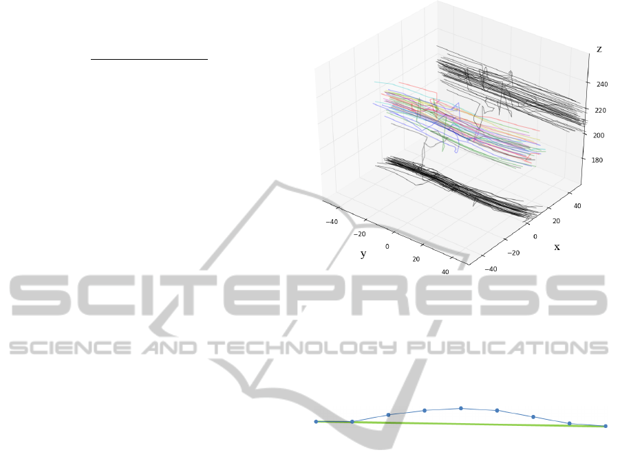
This work presents a method to reconstruct 3D
graphs. A 3D graph is a graph in which every node
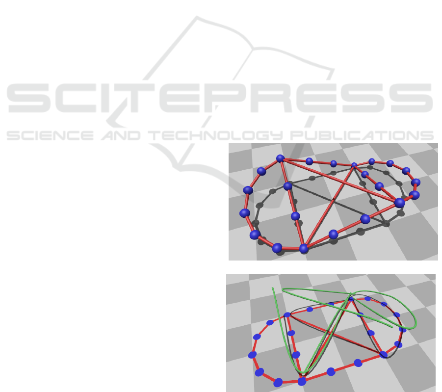
is assigned a position in 3D – as seen in the example
in Figure 1(a). The inputs to the proposed reconstruc-
tion method are shown in Figure 1(b):
1. A 2D orthographic bijective projection of nodes
of the graph – A graph with the same topology,
but with nodes’ positions in 2D. This 2D graph
can be self-intersecting.
2. A set of imprecise 3D positional univariate traces
along the graph’s edges.
Our goal is to estimate the third coordinate of each
node’s position — which will henceforth be referred
to as an elevation. We discuss two variants of the ele-
vation method, both based on registering the traces to
the 2D graph:
The absolute average variant. (AAV) averages the
elevations of the traces at every node.
The relative average variant. (RAV) deduces the
elevations using a first-order differences of the
traces’ elevations.
We argue that the RAV provides results that can be
more robust and precise, under certain conditions. We
also present a method to reconstruct the 3D graph
even when some of it’s nodes are not covered with
any 3D trace. This is achieved based on some addi-
tional assumptions on the structure of the 3D graph.
(a) A 3D graph this work seeks to reconstruct.
(b) Inputs: a 2D projection of the 3D graph and a set of im-
precise 3D traces.
Figure 1: An example of output and inputs for our method.
One clear motivation to the proposed method is
the need for reconstruction of road’s interchanges in
3D. An existing 2D road map serves as a 2D pro-
jection of the desired 3D road graph. GPS traces
recorded while driving through the interchanges pro-
vide the 3D traces of the graph.
13
Hershko N. and Elber G..
3D Graph Reconstruction from 2D Graphs Projections and Univariate Positional Traces in 3-Space - With Application to 3D Reconstruction of Road’s
Interchanges.
DOI: 10.5220/0004652500130021
In Proceedings of the 9th International Conference on Computer Graphics Theory and Applications (GRAPP-2014), pages 13-21
ISBN: 978-989-758-002-4
Copyright
c
 2014 SCITEPRESS (Science and Technology Publications, Lda.)

The rest of the paper is organized as follows. Sec-
tion 2 discusses related work. Section 3 explains the
reconstruction problem in more details and Section 4
describes our proposed reconstruction method. Sec-
tion 5 outlines the application of the method to re-
construction of road’s interchanges from GPSs. In
Section 6, we present results and verification of the
implementation against real ground truth data, and fi-
nally, Section 7 discusses some future work and con-
cludes.
2 RELATED WORK
There are quite a few examples for 3D graphs recon-
struction from imagery data. In the medical field,
Coste et al. presented an algorithm to reconstruct a 3D
blood vessels network from several 2D projections,
acquired from angiographic imaging (Coste et al.,
1999). In the field of GeoInformatics, (Chen et al.,
2006) and others presented methods to reconstruct
3D road models using LIDAR (LIght Detection And
Ranging) data captured airborne.
Reconstruction of graphs from traces was studied
primarily in the context of GeoInformatics — a re-
sult of the prevalence of low-cost GPS receivers, mak-
ing it easy to crowd-source positional traces (Heipke,
2010). While most works focus on reconstruction
of 2D road networks (Cao and Krumm, 2009; Chen
et al., 2010), it has been demonstrated that GPS traces
can also be used to reconstruct a 3D road network
(Guo et al., 2007). However, the main problem of
(Guo et al., 2007) in reconstruction of road networks
is that it results in many cases with a topologically-
inaccurate graphs that need to be manually corrected
(Fathi and Krumm, 2010).
Another general approach for the reconstruction
of 3D graphs from traces considers the input traces
as a graph embedded in a metric space – a “metric
graph” (Kuchment, 2004). The metric graph is sim-
plified using a method suggested, for example, by
(Aanjaneya et al., 2012), and the simplified graph
is then re-embedded in R
3
. It should be noted that
the conversion of traces to a (single connected) met-
ric graph is not natural, and this approach disregards
the connectivity of the points in the traces. Also, the
method presented by Aanjaneya et al. results with a
graph that is guaranteed to be topologically-correct
only for a certain limit of positional error.
3 PROBLEM DESCRIPTION
Let G = (N, E, p) be a 3D (possibly directed) graph,
comprising of a set of nodes N, a set of (possibly
directed) edges E, and position mapping p : N →
R
3
. We will regard the edges as the linear segment
between the corresponding nodes’ positions. The
graph’s 2D projection is denoted
˜
G = (N,E, ˜p), with
˜p : N → R
2
. The unknown vertical component of each
node, N
k
, will be referred to as the node’s elevation
and denoted N
e
k
. In the rest of this work, we will use
k, l and m as indices of nodes.
A trajectory p
i
along the 3D graph is a continuous
arc-length piecewise-linear parameteric curve p
i
(s) :
[0,L
i
] → R
3
of length L
i
∈ R such that p
i
(s) is always
on a graph’s edge, and its derivative p
0
i
(s), if exists,
adheres to the edge’s direction. A trace T
i
over the
3D graph G is a piecewise-linear sampling T
i
= {t
i, j
}
such that t
i, j
= p
i
(s
i, j
)+ d
i
(s
i, j
) ∈ R
3
for some trajec-
tory p
i
(s) : [0,L
i
] → R
3
on the graph and some error
function d
i
(s) : [0, L
i
] → R
3
that is bounded and Lips-
chitz continuous. In the rest of this work, we will use
i as an index of a trace and j as an index of a point in a
trace. The word “node” (or “graph node”) will be ex-
clusively used for elements in N, whereas the points
along some trace will be referred to as “trace points”.
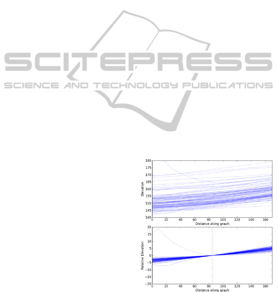
Figure 2 presents an example of the expected be-
haviour of the positional traces, in the ‘z’ axis. As
can be seen from the figure, while the variance of the
positions is quite large, the differences in the change
Figure 2: Elevation profiles of a set of imprecise traces, trac-
ing the same route in the graph (top) and the same traces,
each coerced to zero at the center, exposing the relative dif-
ferences in elevations (bottom).
GRAPP2014-InternationalConferenceonComputerGraphicsTheoryandApplications
14

of elevation are quite small. Given the graph’s 2D
projection
˜
G and a set of such traces T = {T
i
}, in the
next section we present our approach to reconstruct
the graph in 3D — namely, assign each node its ele-
vation.
4 THE METHOD
Assuming the traces’ error functions d
i
are small
enough, we will be able to register each trace to the
route that represents it on the 2D graph, and use aver-
ages of the traces’ elevations as an estimator to the 3D
graph position (The AAV approach). However, if the
error d
i
drifts globally, the entire traces might shift,
while the derivatives will remain quite accurate. In
this case, one rather use the traces’ derivatives as an
estimate to the corresponding edges’ derivative, and
globally resolve them over the graph to estimate the
elevation (the RAV approach).
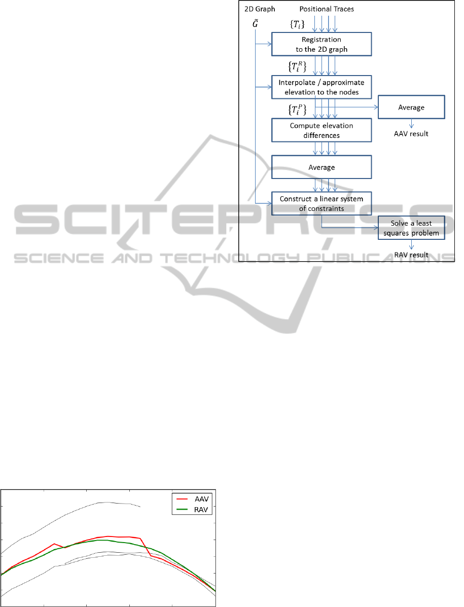
Hence, the method we propose to resolve the 3D
reconstrcution problem includes the following steps:
1. Registration of the 3D traces to the 2D graph.
2.a. (AAV) Averaging the elevations of the nodes of
the 2D graph across all the traces, or ;
2.b. (RAV) Averaging the elevations’ differences on
the edges across the traces, and solving for the
absolute elevations using some known boundary
conditions.
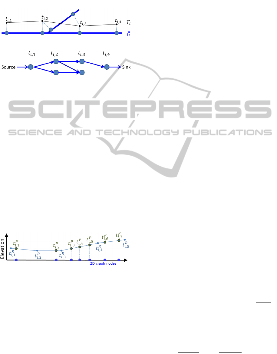
Figure 3 compares the AAV and RAV in a typical re-
construction case for graphs: two of the three traces
are partial (a result of splitting or merging with other
paths in the graph), and they don’t cover all this path.
While the AAV results with a disontinuity, the RAV
results with a smooth solution. Figure 4 provides an
overview of the different steps in our method, and the
different steps are now discussed in detail.
Figure 3: Comparison of the two reconstruction variants on
a synthetic example. The original input traces are shown in
black.
Figure 4: Overview of our method.
4.1 Registration
The registration of the traces correlates every trace
T
i
with the 2D graph
˜
G, resulting with the registered
trace T
R
i
= {t
R
i, j
}, where every point on the trace, t
R
i, j
,
contains the corresponding position on the graph
˜
G
and the edges in the graph to the position of the next
point of the trace, t
R
i, j+1
. The registered trace’s path is
the graph nodes along the trace. It should be noted
that the input trace T
i
is of the same length as its
graph-registered counterpart T
R
i
. The registration can
be done in various methods that consider the traces’
positions and derivatives in relation to the 2D graph,
account for the graph’s topology, or use other domain
knowledge or information that is available in a spe-
cific application.
In this work, we use a simple Map-Matching
method from the field of Geographic Information Sys-
tems, known as Weight-based Map Matching (Yin and
Wolfson, 2004). For every point t
i, j
along the trace,
we find all possible candidate matched points on the
graph, and weigh them based on the distance from the
trace. We then build a candidate graph: The nodes are
the set of all candidate points, and the edges are the
set of shortest paths between pairs of adjacent candi-
date points, directed as in the trace. An example can
be seen in Figure 5. A least-cost path on the graph,
calculated using a Dijkstra’s algorithm, corresponds
to a valid matching of the trace with a minimal total
distance from the graph.
3DGraphReconstructionfrom2DGraphsProjectionsandUnivariatePositionalTracesin3-Space-WithApplicationto
3DReconstructionofRoad'sInterchanges
15

For more information about the various Map-
Matching methods, (Yuan et al., 2010) provide a re-
cent overview, together with their own approach.
(a) The 2D graph
˜
G, a trace T
i
and the candidate points for
the trace points.
(b) Candidate graph.
Figure 5: Construction of a candidate graph for a trace.
4.2 Absolute Average Variant (AAV)
In this reconstruction variant, every node’s elevation
is calculated as a simple average of the elevations of
all traces through it. First, every registered trace T
R
i
is used to calculate the elevations of the graph nodes
in the trace’s path, using some interpolation or ap-
proximation scheme, resulting with T
P
i
= {t
P
i, j
}, such
that N[t
P
i, j
] is the corresponding node in the graph and
e[t
P
i, j
] ∈ R is the node’s interpolated/approximated el-
evation according to this trace. It should be noted
that T
P
i
is usually not of the same length as the regis-
tered trace T
R
i
that it is based upon. Our implementa-
tion is using a linear interpolation of the elevations on
the distance along the trace’s path in the graph, as is
shown in Figure 6.
Figure 6: Constructing T
P
i
using linear interpolation of the
elevation of the registered trace T
R
i
on nodes along its path.
Note that this is done for every trace T
i
, so each node is usu-
ally assigned with more than one elevation – from different
traces.
After calculating the elevations of the nodes along
the traces, e[t
P
i, j
], we simply average the elevations
of each node in the graph. For the sake of brevity,
we will use O(k) to denote the set of all the elevated
nodes (based on the different traces) corresponding to
the node N
k
:
O(k) =

t
P
i, j
: N[t
P
i, j
] = N
k

. (1)
In the AAV, the final elevation of the node N
k
will then
be:
AAV
k
=
1
kO(k)k
∑
t
P
i, j
∈O(k)
e[t
P
i, j
] . (2)
4.3 Relative Average Variant (RAV)
In this reconstruction variant, the interpolated traces
{T
P
i
} are calculated as in the AAV, but are used only
for the first-order elevation differences between ad-
jacent nodes. The elevation differences are averaged
and then globally resolved in the least-squares sense,
over an over-constrained linear system, in which the
unknowns are the nodes’ elevations {N
e
k
}. Let O(k,l)
be the set of all pairs of adjacent elevated nodes on a
trace:
O(k, l) =

(t
P
i, j
, t
P
i, j+1
) ∈ O(k) × O(l)

. (3)
Each such averaged elevation difference over a
graph’s edge is expressed in the linear system as the
constraint:
N
e
k
− N
e
l
=
1
kO(k, l)k
∑
(t
P
i, j
, t
P
i, j+1
)
∈O(k,l)
e[t
P
i, j
] − e[t
P
i, j+1
] . (4)
In additions to the relative elevations, some abso-
lute elevation are also prescribed as boundary condi-
tions.
N
e
k
= BoundaryElevation
k
. (5)
A different weight could be assigned to some con-
straints, representing our confidence in these eleva-
tions’ accuracy.
The RAV also allows us to assign elevation to
nodes that are not covered by any trace. Under
the assumption that the graph’s elevations tend to
change smoothly and gradually, one can assign a zero-
elevation-difference contraints to all edges that have
no elevation difference information:
N
e
k
− N
e
l
= 0 if O(k, l) =
/
0 . (6)
Let N
k
, N
l
, and N
m
be three consecutive nodes in the
graph, such that N
l
is connected only to N
k
and N
m
,
and there is no trace that traverses any of the edges
N
k
N
l
and N
l
N
m
. To obtain a linear elevation change
over these edges, we assign a weight of 1/
p
d(k,l)
to the constraint in Equation (6), where d(k, l) is the
xy length of the graph edge N
k
N
l
. As no other con-
straint depends on N
e
l
, minimizing the energy of the
two weighted constraints
E =
N
e
k
− N
e
l
p
d(k,l)
!
2
+
N
e
l
− N
e
m
p
d(l,m)
!
2
, (7)
GRAPP2014-InternationalConferenceonComputerGraphicsTheoryandApplications
16

with respect to N
e
l
(i.e. differentiating E with respect
to N
e
l
and equating to zero), results with
N
e
l
=
N
e
n
d(k,l) + N
e
k
d(l,m)
d(k,l) + d(l, m)
, (8)
which describes the linear dependency of N
e
l
on its
two neighbors. Repeating the process on pairs of
edges along an “uncovered” path explains the lin-
ear change of the elevation between the two terminal
nodes.
The system of linear constraints formed out of (4),
(5) and (6) is solved in the least-squares sense. As
this is a sparse system, a sparse least-squares solver
such as LSQR (Paige and Saunders, 1982) can be em-
ployed.
5 APPLICATION TO ROAD’S
INTERCHANGES
This section describes the implementation of the pre-
sented method in the specific application of recon-
struction of road’s interchanges in 3D from a 2D road
map and GPS traces.
We used data from the OpenStreetMap project at
http://www.openstreetmap.org/ (Haklay and Weber,
2008) – for both the tagged 2D road map and GPS
traces uploaded by the users.
5.1 Input processing
GPS traces have the property of a global drifting error
as mentioned in the problem description (with time as
the curve parameter). In fact, Figure 2 presents GPS
traces – it consists of GPS traces recorded using the
same device and in the same place, over the course of
several months. However, during the recording, the
user can change his/her speed and can even come to
a stop. As the position of the GPS trace continues
to drift, it results with a significant error over a short
distance. This can be seen in Figure 7. Our proposed
remedy is to remove and split the traces where the
speed is too low – making the error as a function of
the distance small – satisfying the problem’s require-
ments. One should note that in practice this difficulty
is not manifested in interchanges as cars usually drive
at some minimal speed.
We pre-process the 2D road map as well. Long
straight roads are usually represented in Open-
StreetMap as a single segment (consisting of the two
nodes at the extremes). However, in 3D it is often
the case that the road is not straight but has some
vertical alterations. To allows the reconstruction to
express these higher frequency details, we refine all
Figure 7: Several GPS traces recorded with the vehicle
coming to a stop (before a traffic light), and their projec-
tion on the xy and yz planes. Note the large variance in z
compared to xy.
roads so the maximum segment is of bounded length
– as demonstrated in Figure 8.
Figure 8: Side-view of a long road segment (bottom), and
its refinement (top) revealing some elevation curvature.
5.2 Boundary Conditions
As boundary conditions in the RAV, we use the cir-
cumference of the approximated region – where the
calculated road network is stitched to the rest of the
world. We seek to process (i.e. render) the algo-
rithm’s result together with parts of the road’s network
that don’t have an approximated elevation. Hence, all
roads that enter/leave the region under approximation,
will be set with a boundary condition that will force
the stitching to the surroundings, to be continuous.
6 RESULTS AND VERIFICATION
Figure 9 presents a pair of results of the algorithm
using maps and traces from the OSM project. The
road network in these examples was refined based on
a maximum segment length of 30 meters.
In order to validate our approach, we use
the ‘Mesubim’ interchange in Israel, at (32.038N,
34.830E), for which ground-truth data is available.
Figure 10 shows its map and a set of traces over it
3DGraphReconstructionfrom2DGraphsProjectionsandUnivariatePositionalTracesin3-Space-WithApplicationto
3DReconstructionofRoad'sInterchanges
17

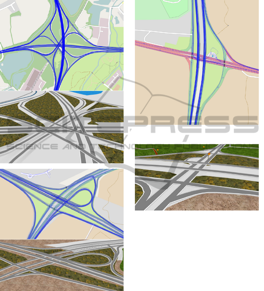
(a) The M4-M25 interchange in the UK (51.495N, 0.495W).
(b) The ‘Morasha’ interchange in Israel (32.124N, 34.855E).
Figure 9: The result of applying the RAV reconstruction
algorithm on some interchanges. Shown are the traces (top)
and the 3D reconstruction (bottom) of both interchanges.
and Figure 11 shows the result of applying the RAV
algorithm to the interchange. This map consists of
601 nodes and 633 edges. 118 traces were processed
into a linear system of 642 constraints, including
274 relative-elevations constraints (Equation (4)), 359
zero-elevation-difference constraints (Equation (6))
Figure 10: The OSM map and the available GPS traces at
the ‘Mesubim’ interchange (32.038N, 34.830E).
Figure 11: The result of applying the RAV reconstruction
algorithm on the interchange in Figure 10.
and 9 boundary conditions Equation ((5)). Matching
the traces to the map took 6 seconds and solving the
least-squares problem took half a second – both on a
single 2.8GHz CPU core. We use ‘ground truth’ el-
evation data that is derived from a photogrammetric
measurement and has an elevation accuracy of 0.3 to
0.5 meters, and horizontal sampling interval along the
roads is in the range of 8 to 15 meters.
Since the OpenStreetMap 2D data does not per-
fectly match, in xy, to the ground truth, the roads’
2D locations were registered manually (with changes
of up to 12 meters – perpendicular to the road direc-
tion) for the sake of this verification. The OSM roads
at this interchange were then resampled at intervals
of one meter, and the elevations resulting from our
algorithms were compared to the elvations at those
uniformly-sampled ‘ground truth’ points.
We compared both presented variants. Note that
while the RAV provides elevation for roads that are
GRAPP2014-InternationalConferenceonComputerGraphicsTheoryandApplications
18

(a)
(b)
(c)
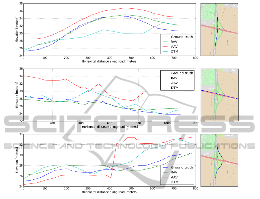
Figure 12: Plots of elevations along several roads of the interchange in Figure 10.
not covered with any trace, the AAV does not. Fig-
ure 12 presents several of the road sections at the in-
terchange, with the elevations along them, including
the ground truth, the results of both the AAV and the
RAV, and elevations derived from a publicly available
Digital Terrain Model (DTM), for comparison. From
Figure 12, several points can be noted:
• Figure 12(a), which depict elevations on the
bridge, have the least agreement between the
ground truth and the DTM (a difference of 4 me-
ters). It seems that due to the low resolution of the
DTM, it only partially captures the bridge’s eleva-
tion details. This can also be seen in Figure 12(b),
which depicts the road under the bridge.
• Since the road in Figure 12(a) have the most GPS
traces, and it is uninterrupted (as there are no traf-
fic lights or other stops along those roads) both
variants yield good agreements with the ground
truth.
• Since Figures 12(b) and 12(c) have low and in-
termittent coverage, the AAV behaves poorly.
Specifically, in Figure 12(c) at the 410m mark,
we leave a road covered by only 2 traces, and go
through several nodes that are covered by many
different traces. However, the RAV continues to
perform well in these cases, taking into account
only elevation differences in traces, and not be-
tween traces.
• In the right side of Figure 12(b), it is visible that
where the AAV has no information, the RAV falls
back to a linear interpolation.
• The RAV was calculated for this intersection on a
larger area than the provided ground truth. There-
fore, the boundary conditions are not set exactly
on the ends of Figures 12 (a) and (b). More so, the
road shown in Figure 12 (c) is even farther away
from the boundaries.
In Figure 13, we see a histogram of the differences
between the ground truth and the results of apply-
ing both variants (in road segments where the AAV
provides a result). These differences’ aggregates are
specified in Table 1. From these results, it is clear
that the RAV yields elevations that are closer to the
3DGraphReconstructionfrom2DGraphsProjectionsandUnivariatePositionalTracesin3-Space-WithApplicationto
3DReconstructionofRoad'sInterchanges
19

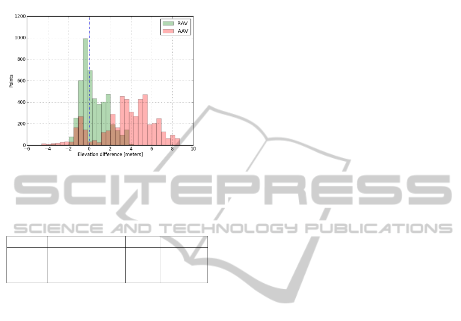
ground truth than the AAV — both in terms of mean
and variance of the difference.
Figure 13: Histograms of the elevation difference between
the tested method variants and the ground truth.
Table 1: A comparison of the different methods’ results to
the ground truth. “coverage” refers to all the points with at
least one trace covering it.
Vatiant Data Mean Variance
RAV all points (6606) +0.59 1.51
RAV coverage (4923) +0.47 1.63
AAV coverage (4923) +3.56 6.88
One should note that since the GPS receiver is typ-
ically not located at the ground level while recording,
it is expected that the AAV will results with some off-
set in z above the ground truth, but this should not
affect the variance of the comparison with the ground
truth.
7 CONCLUSIONS AND FUTURE
WORK
In this paper, we presented an approach for the recon-
struction of 3D graphs from 3D positional traces and
2D graphs, and shown that this method can provide
good results in the application of road interchanges.
We believe that the RAV method might also be ap-
plied to other applications such as medical reconstruc-
tion, cave mapping, or flight paths. In order to adapt
this method to other applications, we suggest a vari-
ation to the problem as follows. Since we use in this
method the graph’s 2D positions only for the purpose
of registering the traces, we could think of a variation
of the problem in which the nodes’ 2D positions are
not known, and instead other information is available
to allow us to register the traces to the graph, or the
2D positions are not accurate but can still be used for
registration. In that case, instead of calculating the
nodes’ elevations, every coordinate of the nodes’ po-
sitions is calculated separately and independently in
the same manner.
For the application of 3D road network recon-
struction from traces, we suggest a semi-automatic
method to provide more topologically-accurate re-
sults than existing methods that reconstruct a road net-
work from traces alone. With the evident success of
OpenStreetMap and other commercial 2D maps, we
believe that using our method on existing 2D datasets
to ameliorate them to 3D can provide with results that
are more robust, due to the high quality of these exist-
ing datasets. In general, the system would consist of
the following steps:
1. Reconstruction of a 2D graph from the univari-
ate traces using an existing 2D reconstruction
method, such as (Guo et al., 2007; Cao and
Krumm, 2009; Chen et al., 2010).
2. Augmentation of the 2D graph into 3D using the
method presented in this work.
This proposed approach also allows one to make use
of traces that have only 2D information in the first
step, and to achieve reasonably good results with a
small amount of 3D traces.
Finally, a more comprehensive data analysis on
the GPS output signal might provide with an ap-
propriate filtration and noise-removal method, which
might improve the reconstruction quality for the in-
terchanges application. Still, the basic property of a
global trace error will still manifest in traces recorded
by consumer devices, and thus the method presented
in this paper or an equivalent method is still required.
ACKNOWLEDGEMENTS
This research was supported in part by the E. and J.
Bishop Research Fund, Technion.
We would also like to thank Armi Grinstein –
Geodetic Engineering Ltd (http://www.armig.co.il/)
for kindly providing us with the ground truth data for
the ‘Mesubim’ interchange.
REFERENCES
Aanjaneya, M., Chazal, F., Chen, D., Glisse, M., Guibas, L.,
and Morozov, D. (2012). Metric graph reconstruction
from noisy data. International Journal of Computa-
tional Geometry & Applications, 22(04):305–325.
Cao, L. and Krumm, J. (2009). From gps traces to a routable
road map. In Proceedings of the 17th ACM SIGSPA-
GRAPP2014-InternationalConferenceonComputerGraphicsTheoryandApplications
20

TIAL International Conference on Advances in Geo-
graphic Information Systems, pages 3–12. ACM.
Chen, D., Guibas, L. J., Hershberger, J., and Sun, J.
(2010). Road network reconstruction for organiz-
ing paths. In Proceedings of the Twenty-First An-
nual ACM-SIAM Symposium on Discrete Algorithms,
pages 1309–1320. Society for Industrial and Applied
Mathematics.
Chen, L.-C., Lo, C.-Y., Shao, Y.-C., and Teo, T.-A. (2006).
Automatic reconstruction of 3d road models by us-
ing 2d road maps and airborne lidar data. In Pro-
ceedings of 27th Asian Conference on Remote Sensing
(ACRS2006), pages 9–13.
Coste, E., Vasseur, C., and Rousseau, J. (1999). 3d recon-
struction of the cerebral arterial network from stereo-
tactic dsa. Medical physics, 26:1783.
Fathi, A. and Krumm, J. (2010). Detecting road intersec-
tions from gps traces. In Geographic Information Sci-
ence, pages 56–69. Springer.
Guo, T., Iwamura, K., and Koga, M. (2007). Towards
high accuracy road maps generation from massive
gps traces data. In Geoscience and Remote Sensing
Symposium, 2007. IGARSS 2007. IEEE International,
pages 667–670. IEEE.
Haklay, M. and Weber, P. (2008). Openstreetmap: User-
generated street maps. Pervasive Computing, IEEE,
7(4):12 –18.
Heipke, C. (2010). Crowdsourcing geospatial data. IS-
PRS Journal of Photogrammetry and Remote Sensing,
65(6):550–557.
Kuchment, P. (2004). Quantum graphs: I. some basic struc-
tures. Waves in Random media, 14(1):S107–S128.
Paige, C. C. and Saunders, M. A. (1982). Lsqr: An al-
gorithm for sparse linear equations and sparse least
squares. ACM Trans. Math. Softw., 8(1):43–71.
Yin, H. and Wolfson, O. (2004). A weight-based map
matching method in moving objects databases. In Sci-
entific and Statistical Database Management, 2004.
Proceedings. 16th International Conference on, pages
437–438. IEEE.
Yuan, J., Zheng, Y., Zhang, C., Xie, X., and Sun, G.-Z.
(2010). An interactive-voting based map matching al-
gorithm. In Mobile Data Management (MDM), 2010
Eleventh International Conference on, pages 43–52.
IEEE.
3DGraphReconstructionfrom2DGraphsProjectionsandUnivariatePositionalTracesin3-Space-WithApplicationto
3DReconstructionofRoad'sInterchanges
21