
Application of Dynamic Distributional Clauses for Multi-hypothesis
Initialization in Model-based Object Tracking
D. Nitti
1
, G. Chliveros
2
, M. Pateraki
2
, L. De Raedt
1
, E. Hourdakis
2
and P. Trahanias
2
1
Department of Computer Science, KU Leuven, Heverlee, BE-3001, Belgium
2
Institute of Computer Science, Foundation for Research and Technology Hellas, Heraklion, Crete, GR-70013, Greece
Keywords:
Object Tracking, Robot Vision, Particle Filters, Distributional Clauses.
Abstract:
In this position paper we propose the use of the Distributional Clauses Particle Filter in conjunction with a
model-based 3D object tracking method in monocular camera sequences. We describe the model based object
tracking method that is based on contour and edge features for 3D pose relative estimation. We also describe
the application of the Distributional Clauses Particle Filter that takes into account inputs from object tracking.
We argue that objects’ dynamics can be modeled via probabilistic rules, which makes possible to predict and
utilise a pose hypothesis space for fully occluded or ‘invisible’ (hidden-away) objects that may re-appear in
the camera field of view. Important issues, such as losing track of the object in a ‘total occlusion’ scenario, are
discussed.
1 INTRODUCTION
Tracking of 3D objects from a monocular camera is
an important problem in service robotics applications
and various approaches have been suggested (Lepetit
and Fua, 2005). Early works utilised 3D CAD mod-
els (Harris, 1992; Koller et al., 1993) and refinement
of the estimated object pose but they do not consider
evaluation and/or prediction of hypothesised object
poses. In fact, most tracking algorithms assume good
pose priors, which can lead to losing track of the ob-
ject in long image sequences.
In effect, the pose hypotheses space is an impor-
tant issue to explore, alongside the use of generated
model feature points which can reduce perspective-
n-point ambiguities in data association (Puppili and
Calway, 2006). In a deterministic setting, (Vacchetti
et al., 2004) employ limited number of hypotheses
and the tracking problem is solved via ‘local’ bundle
adjustment. In a probabilistic setting, large numbers
of pose hypotheses are considered within Sequential
Monte Carlo (SMC) frameworks (Azad et al., 2011).
The issue of ‘re-initialisation’ has been consid-
ered (Choi and Christensen, 2012) for establishing
and generating a higher number of hypotheses (parti-
cles), when degenerate pose estimates occur (e.g. ob-
ject either comes out of the camera frame or is oc-
cluded). However the search space may be too large
to converge to valid pose candidate within reasonable
time. Therefore, key issues in order to not losing track
of the object, given the tracking history, would be to:
• predict the object’s position and spatial relations
when the object(s) is partially or fully occluded,
for long periods of time;
• use of predicted object pose space when the object
becomes ‘invisible’;
• processing time maintains on-line performance.
In this position paper we advocate the use of Dis-
tributional Clauses Particle Filter (DCPF; Section 3)
that utilises a model-based 3D object tracking pro-
cedure (MH3DOT; Section 2). The DCPF predicts
the position of an ‘invisible’ object, whereas the state
transition model is defined with a probabilistic rela-
tional language (Gutmann et al., 2011; Nitti et al.,
2013). The interaction of MH3DOT to and from
DCPF, is sketched in Section 4.
Preliminary results for the described methods, in a
simulated scenario where ground truth data are avail-
able, are presented in Section 5. Concluding remarks
and future work is provided in Section 6.
2 MULTI HYPOTHESES 3D
OBJECT TRACKING - MH3DOT
2.1 Matching and Pose Estimation
Given 3D points from an instance of some pose s from
a known model m
i
we extract the 3D-to-2D projected
feature model points
ˆ
m
i
. The set of model points are
256
Nitti D., Chliveros G., Pateraki M., De Raedt L., Hourdakis E. and Trahanias P..
Application of Dynamic Distributional Clauses for Multi-hypothesis Initialization in Model-based Object Tracking.
DOI: 10.5220/0004654002560261
In Proceedings of the 9th International Conference on Computer Vision Theory and Applications (VISAPP-2014), pages 256-261
ISBN: 978-989-758-004-8
Copyright
c
2014 SCITEPRESS (Science and Technology Publications, Lda.)

matched with image observed feature points
ˆ
p
j
. This
is performed by employing a nearest neighbour search
whereas we query for each model feature points
ˆ
m
i
and find the Euclidean distance for given image ob-
served feature points
ˆ
p
j
using a uniform grid search
subspace. The image observed feature points are pro-
duced from the contour and edges of the model, as per
method described in (Baltzakis and Argyros, 2009)
and further extended in (Pateraki et al., 2013).
Object pose estimation can be performed via point
correspondences C between P = {
ˆ
p
j
} and M =
{
ˆ
m
i
} using a fast nearest neighbour search (Muja
and Lowe, 2009) within an Iterative Closest Point
(ICP) estimation algorithm. However, in the pres-
ence of noise and artifacts resulting, for example,
from a cluttered background, the ICP process can
rapidly deteriorate. This is not the case when using
the Least Trimmed Squares estimator in ICP (TrICP;
(Chetverikov et al., 2005)), since it allows for the two
point sets to contain unequal number of points (i 6= j)
and a percentage of points is offered in a ‘trimming’
operation. The best possible alignment between data /
model sets is found by ‘sifting’ (e.g. sorting) through
nearest-neighbour combinations and ‘trimming’ (e.g.
discarding) the less significant pairs. This is in an at-
tempt to find the subset with lowest sum of individual
Mahalanobis distances, defined as
d
2
i j
= (
ˆ
m
i
−
ˆ
p
j
)
T
(S
m
i
+ S
p
j
)
−1
(
ˆ
m
i
−
ˆ
p
j
) (1)
where S
m
i
is the covariance, thus the uncertainty, on
the position of point feature
ˆ
m
i
; and respectively for
S
p
j
of
ˆ
p
j
, which depends on ‘outliers’ and thus the
feature space.
In practice the (robust) Least Trimmed Squares es-
timator and the ‘trimming operation’ does not elim-
inate presence of outliers. Thus, we apply a non-
linear refinement after the TrICP step to ensure that
the influence of outliers is further reduced; similarly
to (Koller et al., 1993; Fitzgibbon, 2003; Chliveros
et al., 2013).
The minimisation is performed on an objective
function formulated as a sum of squares of a large
number of nonlinear real-valued factors:
ˆ
s
t
= argmin
s
n
∑
i=1
||p
i
− f (s,m
i
)||
2
(2)
where f (·) is the function that projects the 3D
model points to the image plane, according to the
parametrised pose s, at translational terms (r
x
,r
y
,r
z
),
and rotational terms (α
x
,α
y
,α
z
).
2.2 Model-based Hypotheses Space
The non-linear minimisation problem of Equation 2
can be solved via the Levenberg-Marquardt (LM) al-
gorithm. The Jacobians required by LM (Lourakis,
2010) can be formulated analytically by performing
symbolic differentiation of the objective function.
However, to maintain a good solution search space
for matching the reprojected models, we generate
hypotheses over rotations (α
x
+ δα
x
,α
y
+ δα
y
,α
z
+
δα
z
). The term δα can be assigned as dictated by
a number of increment steps (N) over the full rota-
tion range (0,π) of the corresponding axis. We gen-
erate said hypotheses only when the error of the LM
minimisation step (Equation 2) exceeds a predefined
threshold.
3 DISTRIBUTIONAL CLAUSES
PARTICLE FILTERING - DCPF
3.1 A probabilistic Relational Language
for Tracking
From a set of objects that are of a known type and
geometry (e.g. mug, bowl, glass), the procedure de-
scribed in Section 2 can provide the pose, colour and
type of the objects that are visible, thus tracked within
the camera field of view. However, object tracking is
hard if the object is occluded for a long period, e.g.,
when it is inside a box, hidden, or outside the sensor
range. Indeed, if the hidden object reappears in a to-
tally different position, data association will probably
fail. We defined a model that solves this problem us-
ing a relational probabilistic language; i.e. Distribu-
tional Clauses (Gutmann et al., 2011) and its dynamic
extension (Nitti et al., 2013)).
This language is based on logic programming. We
now introduce the key notions. A clause is a first-
order formula with a head and a body. The head is an
atomic formula, whereas the body is a list of atomic
formulas or their negation.
For example, the clause
inside(A,B) ← inside(A,C),inside(C,B)
states that for all A, B and C, A is inside B if A is inside
C and C is inside B (transitivity property). A,B and C
are logical variables.
A ground atomic formula is a predicate applied
to a list of terms that represents objects. For exam-
ple, inside(1,2) is a ground atomic formula, where
inside is a predicate, sometimes called relation, and
1,2 are symbols that refer to objects.
A literal is an atomic formula or a negated atomic
formula. A clause usually contains non-ground lit-
erals, that is, literals with logical variables (e.g.
inside(A,B)). A substitution θ, applied to a clause
or a formula, replaces the variables with other terms.
ApplicationofDynamicDistributionalClausesforMulti-hypothesisInitializationinModel-basedObjectTracking
257

For example, for θ = {A = 1,B = 2,C = 3} the above
clause becomes:
inside(1,2) ← inside(1,3),inside(3, 1)
and states that if inside(1,3) and inside(3, 1) are
true, then inside(1,2) is true. In Distributional
Clauses, the traditional logic programming formal-
ism is extended to define random variables. A dis-
tributional clause is of the form h ∼ D ← b
1
,...,b
n
,
where the b
i
are literals and ∼ is a binary predicate
written in infix notation. The intended meaning of
a distributional clause is that each ground instance
of the clause (h ∼ D ← b
1
,...,b
n
)θ defines the ran-
dom variable hθ as being distributed according to Dθ
whenever all the b
i
θ hold, where θ is a substitution.
The term D, that represents the distribution, can
be non-ground, i.e. values, probabilities or distribu-
tion parameters can be related to conditions in the
body. Furthermore, a term '(d) constructed from the
reserved functor '/1 represents the value of the ran-
dom variable d. Consider the following clauses:
n ∼ poisson(6). (3)
pos(P) ∼ uniform(1, 10) ← between(1,'(n), P). (4)
Clause (3) states that the number of objects n is
governed by a Poisson distribution with mean 6;
clause (4) models the position pos(P) as a random
variable uniformly distributed from 1 to 10, for each
person P such that between(1,'(n),P) succeeds.
Thus if the outcome of n is 2, there will be 2 inde-
pendent random variables pos(1) and pos(2).
A distributional clause is a powerful template to
define conditional probabilities: the random variable
h has a distribution D given the conditions in the
body b
1
,...,b
n
(referred also as body). Furthermore,
it supports continuous random variables in contrast
with the majority of the relational languages. The
dynamic version of this language (Dynamic Distri-
butional Clauses) is used to define the prior distribu-
tion, the state transition model and the measurement
model in a particle filter framework called Distribu-
tional Clauses Particle Filter (DCPF).
Finally, particles x
(i)
t
are interpretations, i.e. sets
of ground facts for the predicates and the values of
random variables that hold at time t. The relational
language is useful for describing objects and their
properties as well as relations between them. Prob-
abilistic rules define how those relations affect each
other with respect to time.
3.2 Relational Model for Object
Tracking
We defined a model in Dynamic Distributional
Clauses where the state consists of the positions and
the velocities of all objects, plus the relations between
them. The relations considered are left, right, near,
on, and inside plus object properties such as color,
type and size. We also modeled the following physi-
cal principles in the state transition model:
Property 1 if an object is on top of another object, it
cannot fall down;
Property 2 if there are no objects under an object,
the object will fall down until it collides with an-
other object or the floor;
Property 3 an object may fall inside the box only if
it is on the box in the previous step
Property 4 if an object is inside a box, its position
follows that of the box.
As an example consider property (3). If an object ID
is not inside another object and is on top of a box B,
then it can fall inside the box with probability 0.3 in
the next step. This can be modelled by the following
clause:
inside
t+1
(ID,B)
x
∼ finite([0.3 :true, 0.7 : false]) ←
not('(inside
t
(ID, )) = true),on
t
(ID,B),
type(B,box). (5)
That is to say, a particle at time t with two
objects 1 and 2, where on
t
(2,1),type(1,box),
type(2,cup),'(inside
t
(2,1)) = false hold; the
body of clause (5) is true for θ = {ID = 2,B =
1}, therefore the random variable inside
t+1
(2,1)
at time t + 1 will be sampled from the distribution
[0.3 :true,0.7 :false].
Furthermore, if A is inside B at time t, the relation
holds at t + 1 (clause omitted). If an object is inside
the box, we assume that its position is uniformly dis-
tributed inside the box:
pos
t+1
(ID)
x
∼ uniform('(pos
t+1
(B))
x
− D
x
/2,
'(pos
t+1
(B))
x
+ D
x
/2)) ←
'(inside
t
(ID,B)) = true,size(B,D
x
,D
y
,D
z
). (6)
We only showed the x dimension and omitted the ob-
ject’s velocity for ease of exposition. To model the
position and the velocity of objects in free fall we use
the rule:
pos vel
t+1
(ID)
z
∼ gaussian
"
'(pos
t
(ID))
z
+ ∆t '(vel
t
(ID))
z
− 0.5g∆t
2
'(vel
t
(ID))
z
− g∆t
#
,cov
← not('(inside
t
(ID, ))= true), not(on
t
(ID, )). (7)
It states that if the object ID is neither ‘on’ nor ‘in-
side’ any object, the object will fall with gravitational
acceleration g, where we specify only the position
and velocity for the coordinate z. For the coordinates
VISAPP2014-InternationalConferenceonComputerVisionTheoryandApplications
258
x and y the rule is similar but without acceleration.
The gravitational force can be compensated by a hu-
man or a robot that holds the object. Therefore, the
gravitational acceleration is considered with a certain
probability, whereas the relative clause is omitted for
brevity. The measurement model is the product of
Gaussian distributions around each object’s position
pos
t
(i) (thereby assuming that the measurements are
i.i.d.):
obsPos
t+1
(ID) ∼ gaussian('(pos(ID)
t+1
), cov).
We also need to model that if an object is inside a box,
it will remain inside as long as we do not observe the
object again. Furthermore, the state is extended with
the position and the velocity of an object whenever a
new object is observed (clauses omitted for brevity).
4 DCPF / MH3DOT
INTEGRATION
The proposed approaches (Sections 2, 3) need to be
effectively integrated. The way they interact can have
a significant impact on performance. In this section
we describe the proposed approach.
The MH3DOT pose values and object class are the
observations provided to the DCPF with the described
model. When a new object is detected and tracked by
MH3DOT, the observation needs to be associated to
either an existing or new object in the state of DCPF.
This is known as the data association problem. It can
be solved by adding data association hypotheses in
the state space of the particle filter. This approach is
called ‘Joint Particle Filter’ (De Laet, 2010), though
other solutions are possible.
We assume that the object’s track produced by
MH3DOT (from appearing to disappearing from cam-
era’s field of view) is generated by a single object.
Therefore a data association hypothesis consists of a
set of assignments, whereas an object track is linked
to an object in DCPF state. When an object is no
longer visible, the DCPF estimates its position ac-
cording to the described state transition model. For
example, if an object is inside a box it will follow the
position of the box, and if an object is on top of an-
other, it can either ‘fall down’ or remain on top of the
object.
This allows for tracking objects that may return
within the camera field of view. For example, if an
object is inside a box, and the box is moved, the fil-
ter estimates that the object position follows the box.
Hence, when the tracker detects a new object near the
box, it can be considered as the same object with high
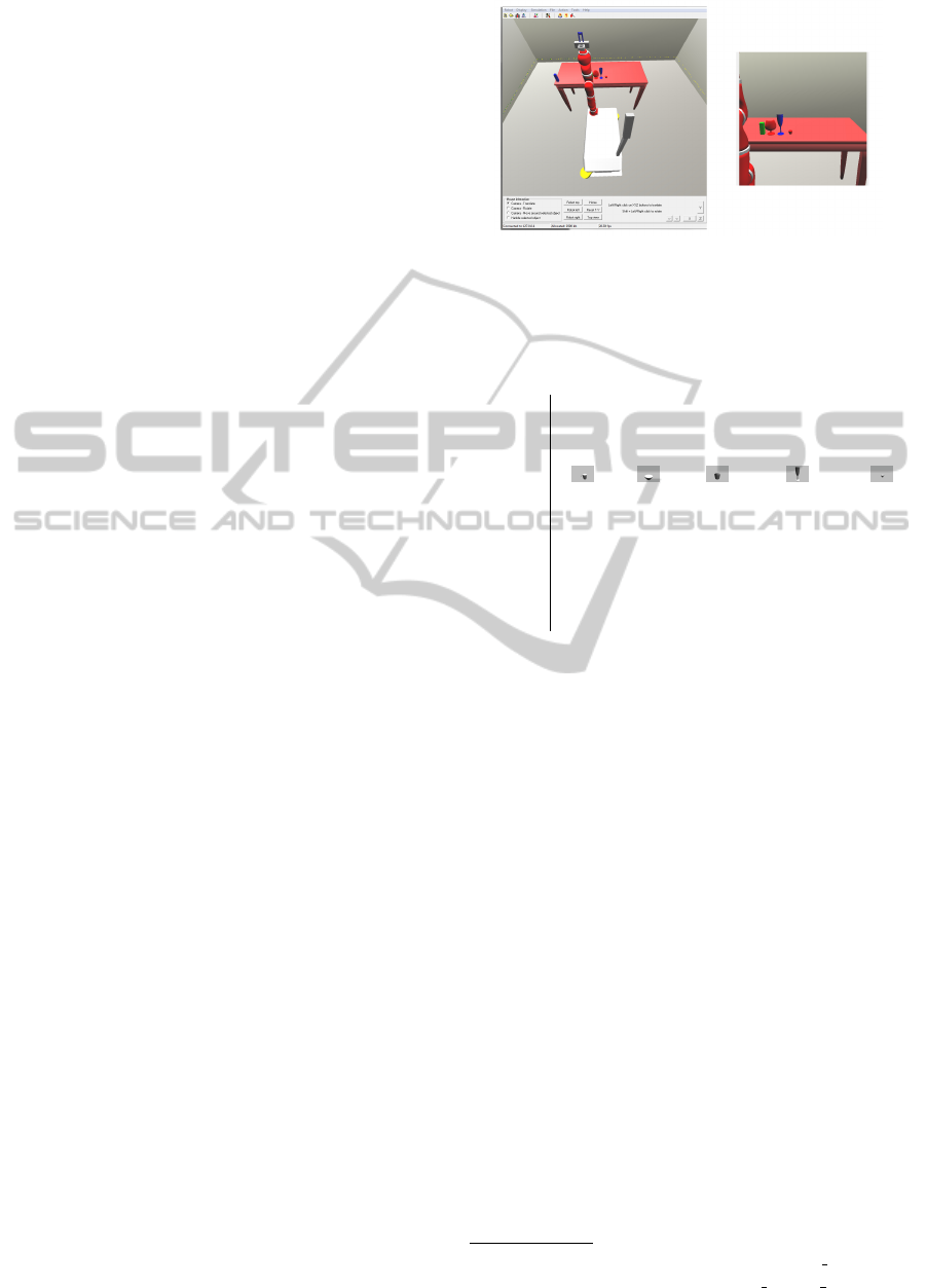
Figure 1: The simulated environment: (left) the robot envi-
ronment setup; (right) instance of simulated camera output.
Table 1: Quantitative evaluation for the accuracy of the
MH3DOT approach. E
·
denotes the mean squared error
from ground truth values: E
d
is in cm and E
φ
x
, E
φ
y
, E
φ
z
is in degrees.
(a) (b) (c) (d) (e)
Model Mug Bowl Glass C. Flute E. cup
E
d
2.8 1.8 2.1 1.2 4.1
E
φ
x
3.1 2.3 3.2 1.2 4.0
E
φ
y
3.2 1.9 1.5 1.2 3.1
E
φ
z
5.6 - - - 6.5
probability. Therefore, tracking the object can be suc-
cessfull even if the object is invisible for long periods
of time; even if re-appearing in a totally different than
the last known position.
5 RESULTS
To quantitatively evaluate the accuracy of the meth-
ods proposed in this paper with respect to the tracking
approach, we have used an environment in a custom
simulator
1
. For the MH3DOT, we have assumed five
simulation sequences using ROS’s household objects
database
2
. For the DCPF, we have used simulated se-
quences where the objects in question appear / disap-
pear from the simulated camera’s field of view.
In what follows, each of the methods is tested
in fully controlled settings (simulation environment;
Figure 1) in order to extract ground truth and have a
valid visible comparison. The former relates to track-
ing accuracy (MH3DOT, Table 1) and the latter to pre-
dictive capabilities (DCPF, Figure 2).
1
http://www.youtube.com/watch?v=-AV0iY u2F4
2
http://www.ros.org/wiki/household objects database
ApplicationofDynamicDistributionalClausesforMulti-hypothesisInitializationinModel-basedObjectTracking
259
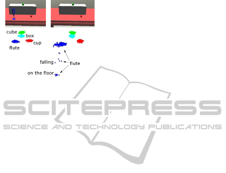
Figure 2: Resulting DCPF prediction (particles’ position
cloud) for a ‘flute’ free-fall from simulated world table.
Evaluation of MH3DOT
Testing for MH3DOT consists of 5 simulated se-
quences. Each sequence consisted of 200 frames, de-
picting a single object from the database which was
located on a flat surface (a table in the simulated
world; see Figure 1). The simulated camera was man-
ually stirred around the object and the relative pose of
the camera with respect to the object was recorded
and used as ground truth.
The proposed algorithm was allowed to run a lim-
ited number of minimisation iterations for each frame
and for a hard coded max number of hypotheses.
The results of MH3DOT are summarized in Table 1,
where each column contains the results of a sequence,
which involves the specific object. E
d
is the average
error (in cm) for the camera-to-object distance and
E
φ
x
, E
φ
y
and E
φ
z
are the average errors (in degrees)
for the rotation angle around each of the x, y, and z
axes of the object. Note that for objects (b),(c) and
(d), no results can be obtained for the rotation around
the z (vertical) axis. This is due to symmetry around
corresponding axis. Also note, that we selected these
objects on purpose because objects of symmetry are
in principle more difficult to track due to their similar
shape from different viewpoints.
Evaluation of DCPF
We tested the DCPF, with the described model, in the
aforementioned simulated environment (as per Fig-
ures 1, 2). The simulated ‘world’ contains four ob-
jects placed on the simulated robot world’s table. In
effect, and with reference to Figure 2, there is a ‘box’
placed on the world table. On top of the box there is a
small toy green ‘cube’, with another two ROS objects
placed on the flat surface of the world table; i.e. the
‘flute’ of colour blue and the ‘cup’ of colour red.
The experiment proceeds by simulated actions
that move objects and remove them from the camera
field of view. We test to see whether the DCPF will
correctly predict positions for the database objects,
given the properties and conditions of the DCPF.
The DCPF correctly estimates the positions (and
relations) of invisible objects in several cases. Fig-
ure 2 shows the simulated camera frames and the pre-
dicted positions (particles; hypothesis space) imme-
diately below each image frame. Each predicted po-
sitions’ particle cloud (coloured dot for each parti-
cle) corresponds to the object’s colouring (e.g. the
blue flute object corresponds to the blue predicted po-
sitions’ particle cloud). For example, Figure 2 left
frame green cube, if it falls inside the box (becoming
invisible) DCPF estimates that it is inside the box or
still on top of the box. If we move the box the esti-
mated object’s position follows the box.
In the illustrated example, we tested the case of an
object being dropped from the table (no longer visi-
ble). This is the case with the ‘flute’ of Figure 2 (left),
that disappears after some frames in Figure 2 (right).
The model predicts that the object is ‘on’ the table,
or ‘falling’ down (less likely) or somewhere ‘on the
floor’ (more likely); see annotation of Figure 2.
6 DISCUSSION
In this position paper we have suggested a new way
for combining predictive capabilities (DCPF) within a
multiple hypotheses methodology (MH3DOT). That
is to say, sampling association variables according to
the state in the DCPF and observations in MH3DOT.
The incorporation of DCPF helps to constraining the
problem of losing track of the object, if it was to
‘disappear’ for long periods of time. The results for
DCPF indicate that it correctly predicts and infers
possible positions (particle clouds) for an object that
is no longer in the camera field of view. The current
work, gives us increased confidence on the validity of
this combined methodology.
In future works we intend to directly address the
data association problem. We further aim to testing
in both simulated and real environments; in particu-
lar, for grasping scenarios via semantic queries. That
is, via a relational language (such as distributional
clauses) it is possible to perform high-level queries;
e.g. list of red objects on the table near a glass, with
the relative probability. This will become the basis for
publishing a fully integrated approach alongside new
results.
VISAPP2014-InternationalConferenceonComputerVisionTheoryandApplications
260

ACKNOWLEDGEMENTS
This work was partially supported by the European
Commission under contract number FP7-248258
(First-MM project). Davide Nitti is supported by the
IWT (Agentschap voor Innovatie door Wetenschap en
Technologie) in Belgium.
REFERENCES
Azad, P., M
¨
unch, D., Asfour, T., and Dillmann, R. (2011).
6-DoF model-based tracking of arbitrarily shaped 3D
objects. In IEEE Int. Conf. on Robotics and Automa-
tion, pages 5204–5209.
Baltzakis, H. and Argyros, A. (2009). Propagation of pixel
hypotheses for multiple objects tracking. In Advances
in Visual Computing, volume 5876 of Lecture Notes
in Computer Science, pages 140–149.
Chetverikov, D., Stepanov, D., , and Krsek, P. (2005).
Robust euclidean alignment of 3D point sets: the
trimmed iterative closest point algorithm. Image and
Vision Computing, 23:299–309.
Chliveros, G., Pateraki, M., and Trahanias, P. (2013). Ro-
bust multi-hypothesis 3D object pose tracking. In Int.
Conf. on Computer Vision Systems.
Choi, C. and Christensen, H. I. (2012). Robust 3D vi-
sual tracking using particle filtering on the special Eu-
clidean group: A combined approach of keypoint and
edge features. The International Journal of Robotics
Research, 31(4):498–519.
De Laet, T. (2010). Rigorously Bayesian Multitarget Track-
ing and Localization. PhD thesis, Katholieke Univer-
siteit Leuven.
Fitzgibbon, A. (2003). Robust registration of 2D and
3D point sets. Image and Vision Computing,
21(13):1145–1153.
Gutmann, B., Thon, I., Kimmig, A., Bruynooghe, M., and
De Raedt, L. (2011). The magic of logical inference
in probabilistic programming. Theory and Practice of
Logic Programming.
Harris, C. (1992). Tracking with rigid objects. MIT press.
Koller, D., Daniilidis, K., and Nagel, H. (1993). Model-
based object tracking in monocular image sequences
of road traffic scenes. International Journal of Com-
puter Vision, 10:257–281.
Lepetit, V. and Fua, P. (2005). Monocular model-based 3D
tracking of rigid objects: a survey. In Foundations and
Trends in Computer Graphics and Vision, pages 1–89.
Lourakis, M. (2010). Sparse non-linear least squares opti-
mization for geometric vision. In European Confer-
ence on Computer Vision, pages 43–56.
Muja, M. and Lowe, D. G. (2009). Fast approximate near-
est neighbors with automatic algorithm configuration.
In Int. Conf. on Computer Vision Theory and Applica-
tions (VISAPP), pages 331–340.
Nitti, D., De Laet, T., and De Raedt, L. (2013). A particle
filter for hybrid relational domains. In IEEE/RSJ In-
ternational Conference on Intelligent Robots and Sys-
tems (IROS 2013).
Pateraki, M., Sigalas, M., Chliveros, G., and Trahanias, P.
(2013). Visual human-robot communication in social
settings. In IEEE Int. Conf. on Robotics and Automa-
tion.
Puppili, M. and Calway, A. (2006). Real time camera track-
ing using known 3D models and a particle filter. In
IEEE Int. Conf. on Pattern Recognition.
Vacchetti, L., Lepetit, V., and Fua, P. (2004). Stable real-
time 3D tracking using online and offline information.
IEEE Transactions on Pattern Analysis and Machine
Intelligence, 26:1385–1391.
ApplicationofDynamicDistributionalClausesforMulti-hypothesisInitializationinModel-basedObjectTracking
261
