
Multilevel Group Analysis on Bayesian in fMRI Time Series
Feng Yang
1
, Kuang Fu
2
and Ai Zhou
3
1
School of Computer Science & Technology, Heilongjiang University, Harbin, Heilongjiang, China
2
The Second Affiliated Hospital of Harbin Medical University, Harbin, Heilongjiang, China
3
College of the Humanities, Jilin University, Changchun, Jilin, China
Keywords: fMRI Time Series, Classical Statistics, Bayesian Inference, Group Analysis.
Abstract: This paper suggests one method to process fMRI time series based on Bayesian inference for group analysis.
The method uses multilevel divided by session, subject and group as pair comparison to reinforce posterior
probability in group analysis from single subjects as priors. And also it combines classical statistics, i.e., t-test
to obtain voxel activation at subject level as prior for Bayesian inference at group level. It effectively solved
computation expensive and complexity. And it shows robust on Bayesian inference for group analysis.
1 INTRODUCTION
In the past decades, functional Magnetic Resonance
Images (fMRI) technology has been obtained greatly
attention all over the world, especially in brain
science field. Most researches have explored brain
principles from the structural to effective
connectivity. Especially for clinical, fMRI would
provide more help for diagnosis and curing brain
diseases, e.g., Alzheimer’s disease, depression,
schizophrenia, sclerosis and non-communicative
brain damaged patients (Margulies et al., 2010).
Functional MRI is a non-invasive technique for
studying brain activities (Lindquist, 2008). It
analyses blood oxygen level dependent (BOLD)
hemodynamic response to identify brain activation
by stimulus. It characters hemodynamic response
function (HRF) to measure brain spatial distribution
based on BOLD signals about neural activity by
vascular hemodynamic changing. The goal of fMRI
analysis is to detect, in a robust, sensitive and valid
way, those parts of the brain that show increased
intensity at the points in time that stimulation was
applied (Smith and Dphil, 2004). They include
functional segregation, functional connection and
effective connectivity.
Most analysis methods of fMRI data are divided
into two categories: model driven and data driven.
For model driven, commonly it uses traditional
statistics methods to measure fMRI data time series.
For data driven, it is based on image density to
compute distance, similarity or features, e.g., Cluster
analysis, Independent Component Analysis (ICA)
and self-organization mapping etc. Statistics
methods are based on a general linear model (GLM)
model to estimate parameter for each voxel and
compute p-value, under null hypothesis and obtain
p-value probability distribution mapping. And then it
maps the probability of each voxel for whole brain
to make statistics parameter mapping (SPM). Due to
issues on classical method, for instance, it never
rejects alternative assumption meaning activation
always occurred, and has false positive ratio (FDR)
for multiple comparison problems. On the contrary,
alternative method is Bayesian which can give the
probability that the effect is greater than some
threshold under voxel activation to avoid above
issues.
In Bayesian theory, the posterior distribution
captures all information inferred from the data about
the parameters. As such (Woolrich, 2012) it
proposed the first Bayesian group inference
approach using a hierarchical model. Bayesian uses
high-level estimation as prior and then enable
posterior inferences of the parameters in low-level.
Then inference is based on the posterior distribution
of the parameters from given the data.
This paper suggests a multilevel Bayesian
inference for group analysis based on hierarchical
model. The multilevel group method is proportional
to multiple levels according to session level, subject
level and group level with comparing individual
91
Yang F., Fu K. and Zhou A..
Multilevel Group Analysis on Bayesian in fMRI Time Series.
DOI: 10.5220/0004655000910097
In Proceedings of the 9th International Conference on Computer Vision Theory and Applications (VISAPP-2014), pages 91-97
ISBN: 978-989-758-009-3
Copyright
c
2014 SCITEPRESS (Science and Technology Publications, Lda.)

subjects as selected prior. We use classical statistics
and Bayesian 1
st
level to compare variances to
inspect prior for individual subjects. Through
different subjects, it passes the estimated parameters
from session level parameters in one subject as prior
to compute posterior of next subject. For group level
analysis, it uses the effects of single subject as prior
to provide next subject analysis based on Bayesian
posterior probability. This can reduce computation
cost and complexity.
For the paper structure, section II describes
Bayesian inference theory and estimation in
multilevel group analysis. Section III shows an
fMRI case analysis with lower level of individual
subject as prior and passing statistics value to higher
level of group. In the last part we specify Bayesian
methods for fMRI dynamic analysis in the future.
2 BAYESIAN METHODS
Bayesian statistics approach is to use conditional or
posterior inference based upon the posterior
distribution of the activation by observed data. A
fully Bayesian statistics approach as the first paper
considered the full posterior probability distribution
was appeared in 1998 (Woolrich, 2012).
In (Friston et al., 2002a, 2002b), it describes
Bayesian on hierarchical linear model to form first
level recursively. And it combines hierarchical
model with classical and Empirical Bayesian, called
all in one (Woolrich et al., 2004), to show two
methods based on the same principle by covariance
components and EM.
For group analysis based on Bayesian, most
methods relay on prior selection. Usually prior is
from temporal or spatial perspectives, or both of
observed data. Temporal prior is commonly
designed by hierarchical model divided into session
level, subject level and group level under two levels.
In (Woolrich et al., 2004, Beckmann et al., 2003),
they use two levels and fully Bayesian framwork,
passing summary statistics from first level to second
level. And also in (Neumann and Lohmann, 2003) it
gives different relation between subject level and
group level according to Bayesian principles guided
by (Box and Tiao, 1992). It passed a random subject
as prior to estimate parameters for other subjects. In
(G’omez-laberge et al., 2011) it uses Bayesian to
cluster analysis which proposes a Bayesian
hierarchical model to describe the correlation
structure of the observed voxel clusters. For spatial
prior, some use regions or areas (Lei et al., 2009) in
Brain to characterize the spatial features of the HRF
over the regression coefficients (Penny et al., 2003).
And in (Ahn et al., 2011), it demonstrated that
hierarchical Bayesian analysis outperforms
conventional maximum likelihood estimation in
recovering true parameters no matter individual or
group analysis.
As (Woolrich, 2012) showing the all procedures
of Bayesian in fMRI analysis, Bayesian methods
become popular method as statistics inference about
activation voxels and group analysis. Through the
above analysis on group methods based on Bayesian,
we combine Bayesian with hierarchical linear model
to estimate parameters from observed data by EM
algorithm. And about prior selection, we suggest that
prior is selected from comparing different individual
subjects analysed by classical method and Bayesian
level.
2.1 Model
For groups analysis, we may construct different
levels from session, cluster, subject and group
perspectives. As shown in Figure 1, we can divid
data into hierarchical levels by the session, subject
and group levels.
We accept hierarchical linear model to construct
parameters among groups including session-level
and group-level. According to the hemodynamic
response with observed data under stimulus, the
hierarchical linear model is defined for individual
subject as below Equation (1).
.
.
.
=
…
…
……
…
.
.
.
.
.
.
(1)
The equation is consisted by three parts:
observed data Y which includes each voxel time
series with n scans, design matrix X which has
contrast regression coefficients with interest and
error. And also it uses β to describe amplitude as
parameters of explanatory.
VISAPP2014-InternationalConferenceonComputerVisionTheoryandApplications
92
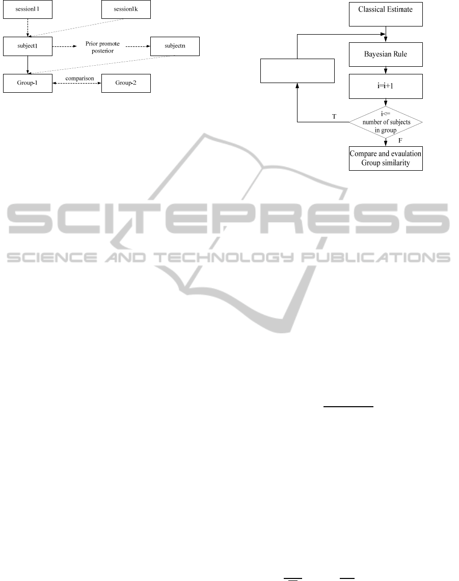
Figure 1: Group hierarchical components.
In group analysis, these subjects have the same
scanning environment and also have similar
background, i.e., age, gender, education, health.
Through these similarities of group, we assume that
they have similar contrast regression of interest
effects. It shows Hierarchical linear model as below
equation (2) for group analysis.
.
.
.
.
.
.
.
.
.
.
.
.
…
…
……
…
.
.
.
.
.
.
.
.
.
.
.
.
.
.
.
.
.
.
.
.
.
.
.
.
(2)
The equation (2) describes one group with m
subjects, single subject with n scans and each subject
with different estimated parameters and errors.
For fMRI data, Bayes directly obtains posterior
distribution of parameters combined prior with
observed data under unknown parameters and easily
to compute the probability of parameters by
Bayesian rules. For prior unknown, the estimation
processing is referred to as empirical Bayes
(Ashburner et al., 2003). And inference is based on
the posterior distribution of the parameters given the
data (Morris, 1983; Casella, 1985). According to the
Bayesian inference based on hierarchical linear
model, the procedure of computation in details is
shown as Figure 2.
Figure 2: Multilevel group analysis procedures.
These priors can be estimated from given the
data and we have multiple subjects of the effect
interested explanatory variants. Bayesian uses
high-level estimate as prior and then enable posterior
inferences about the parameters in low-level by
Bayesian rule.
2.2 Bayesian Rule
According to the two levels model, we use Bayesian
rule to reduce posterior probability distribution by
prior distribution. Bayesian is to calculate the
posterior distribution by prior information and some
new observed data on the first level. By Bayes’ rule,
the posterior of data y is given by equation (3):
p
θ
|
y
|
(3)
Where
py|θ is marginal likelihood or
evidence and pθ as prior. As
be
known,
Bayesian rule becomes the equation (4):
p
θ
|
y
∝p
y
|
θ
∗p
θ
(4)
All marginal likelihood functions have the same
distribution as prior distribution fitting to normal
distribution. At first, according to the prior
distribution as normal distribution θ~Nμ,
, it
gives
pθ and pθ|y likelihood functions as
below (5).
p
y
|
θ
(
√
exp{-
∑
2
}
(5)
And about prior with normal distribution is
shown in (6):
1
(1)
0
i
)|(
)(
yp
i
)(
)(
i
p
MultilevelGroupAnalysisonBayesianinfMRITimeSeries
93

p
θ
=
√
exp
(6)
Putting together, we obtain the P(θ|y) probability
density function in (7). In details reduction, it is
specified at (Box and Tiao, 1992).
p
θ
|
y
/
√
2
exp
1
2
̅
(7)
With the mean ad variance are shown as below
(8).
̅
1
(8)
Combining the hierarchical linear model with
Bayesian rule in group, it has basic formulation as
below (9).
θ
,
,
…,
,
,
…,
∝
θ
∏
|
∝
θ
|
,
,
…,
|
(9)
This reduction is from (Bradley, 1996). Thus, it
combines all formulations into multilevel in group
analysis to show posterior and prior relation as (10).
|
|
∝
|
(10)
For prior selection, some suggest spatial prior
(Penny et al., 2005) and some use wavelet
coefficients as prior (Sanyal and Ferreira, 2012). As
like Stephan (Neumann and Lohmann, 2003)
described, “Today’s posterior is tomorrow’s prior”
which we use the rule as one subject parameters as
prior for next subject in group analysis to decrease
computation cost and complexity.
2.3 Estimation
We use an empirical Bayes methodology to estimate
the hyperparameters which are shared by all subjects.
Parametric empirical Bayes can be formulated
classically in terms of covariance component
estimation (e.g. within subject vs. between subject
contributions to error) (Morris, 1983; Casella, 1985).
Through P(θ|y), we estimate posterior mean and
posterior covariance. To estimate the covariance
components, many different computation methods
are used, for example, some use point estimation,
some use maximum a posterior probability (MAP)
with MCMC under numerical integration
unavailable. In (Friston et al., 2002b), it uses EM
algorithm to estimate error and prior covariance. It
has two basic steps in EM algorithm as equation (11).
For two steps, one is E-step and the other is M-step.
E-step:
Q
θ
log
|
|,
M-step:
|
(11)
E-step computes likelihood function according to i
th
effect or initial value by the first subject and M-step
makes likelihood function maximum to obtain new
parameters. And iteratively it obtains estimator
through the two steps iteratively until convergence.
2.4 Inference
This section describes the construction of posterior
probability maps that enable conditional or Bayesian
inferences about regionally-specific effects in
neuroimaging. All the procedure is focused on
posterior probability computation. At the same time,
Bayesian inference requires prior known or
unknown estimated from given data. This posterior
density can be computed, under Gaussian
assumptions, using Bayes rules.
Posterior probability maps (PPMs) are images of
the probability or confidence that activation exceeds
some specified threshold, given the data. PPMs
require the posterior distribution of a contrast of
conditional parameter estimates by given the data
(Ashburner et al., 2003). It will make mean as
Bayesian estimator to compute p by the equation
(12).
P=1-Ф
|
|
(12)
.
is the cumulative density function of the
unit normal distribution (Friston and Penny, 2003).
An image of these posterior probabilities constitutes
a PPM. According to the p-value, it will map PPMs
to show the activation distribution about voxels on
confidence 95%. The probability that activation has
occurred, given the data, at any particular voxel is
the same (Friston and Penny, 2003).
At the first level of the hierarchy, it corresponds
to the experimental effects at session-level and
obtains the probability of voxel activation. And at
VISAPP2014-InternationalConferenceonComputerVisionTheoryandApplications
94

the second level of the group, it comprises the
effects over subjects through the first level of the
individual subject effects. We describe the Bayesian
inference procedure shown in Figure 3.
Figure 3: Bayesian inference with PPMs procedure.
3 EXPERIMENT
3.1 Data Collection
In this experiment, we choose the dataset which
consists of 24 contiguous slices, 64×64×24 in each
volume with 2×2×2 mm
3
voxels in thickness 5mm in
whole brain BOLD response acquired using 3.0T
fMRI system. For block design, it includes blocks of
6 scans with 12 blocks by removing the first 6 scans
in TR 2s. We design the task with the condition for
successive blocks alternated between rest and visual
picture stimulation from the beginning of rest.
3.2 Preprocessing
During scanning for fMRI data, although usually
subject is required to fix in a frame to avoid motion
to reduce images artifacts, due to machine heating
effects, physical effects as cardiac and respiration,
and moving from subjects, these images from
scanning include some noises. Some noises from
machine heating with high frequency are eliminated
by high frequency filters and some artifacts from
motion can be corrected by preprocessing.
The key issues of preprocessing in SPM are
mainly involved: (1) realignment: It completes
motion correct by align images according to the first
image in the each session and align other sessions
according to the first session; (2) coregistration:
Match images from same subject but different
modalities by coregistration. It supplies mean images
in data to register structural image solving
consistence between functional images and structural
images; (3) segmentation: It segments structure T1*
image to grey matter, white matter and CSF. And it
obtained some parameters for normalize functional
images; (4) normalization: Make results from
different studies compared by aligning them to
standard space it can deal with different Talairach
problems. It normalizes functional images onto
template images, for example, EPI template; (5)
smoothing: Through removing lower frequency
noises, it extends larger spatial SNR in spatial
overlap by blurring over minor anatomical
differences and registration errors; Smoothing can
average neighbouring voxels suppresses noise and
increase sensitivity to effects of similar scale to
kernel.
For our experiment, we choose realignment and
normalize to reduce motion artifacts and make data
being consistence. And also we use classical
inference which needs smoothing as preprocessing to
improve SNR; we separate data without smoothing
for Bayesian 1
st
level.
3.3 Results
Efficient computation at the second-level requires
full access to the first-level parameter estimates and
associated covariance. This involves both the
variances of the parameter estimates and the
covariance between different parameters.
PPMs show posterior probability p value about
activation in group analysis. According to the
activation, is given the results in PPMs which plot a
map of effect sizes at voxels where it is 99% sure
that the effect size is greater than 2% of the global
mean. And it compares the similar covariance
among group in Table 1.
Table 1 is arranged columns which are from right
to left as: (i) region of interest; (ii) voxel-level
t-value; (iii) Z-value; (iv) means; and (v) standard
deviate. The maximum intensity projection (MIP) of
the statistical map is displayed (Friston,
2002).Throughout the Figure 4, it is shown the fitted
response through even-relative response results
among some subjects. With the activation on voxels
for individual subjects, we can compare different
MultilevelGroupAnalysisonBayesianinfMRITimeSeries
95
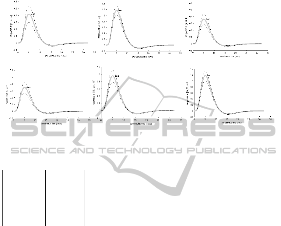
Figure 4: Comparison event-relative response among group.
Table 1: Group Bayesian estimate by prior iterative from
all subjects.
Region (ROI) t Z mean
Standard
deviate
L Heschl gyrus 3.54 3.42 0.32 0.02
R Heschl gyrus 3.49 -3.83 -0.35 0.02
L hippocampus 4.20 4.54 0.16 0.01
R hippocampus 4.34 -4.20 -0.11 0.01
Loccipital gyrus 3.23 3.34 0.13 0.01
Roccipital gyrus 3.45 -4.12 -0.12 0.01
subjects in the group with similar variances and then
we can choose the some subjects as priors for next
group computation.
5 CONCLUSIONS
Any approach to variance estimation can easily be
combined with the multilevel GLM to provide a
practical multilevel method (Beckmann et al., 2003).
Indeed, Bayesian approaches present the significant
effects by combination hierarchical model with
posterior probability. And we can set prior as
multiple levels by comparing subjects as prior in
group analysis to increase computational speed and
more precise effects.
All the above ideas would be the objectives for
next research hot points. Furthermore, Bayesian
would be served for brain science.
ACKNOWLEDGEMENTS
Sponsored by Heilongjiang Province Natural Fund
(F201234) and Science, Technology Research
Project in Heilongjiang Province Department of
Education (12521431) and CSC.
REFERENCES
Ahn Woo-Young, Krawitz Adam, Kim Woojae,
BusemeyeJerome R. r, and Brown Joshua W., 2011. A
Model-Based fMRI Analysis with Hierarchical
Bayesian Parameter Estimation. Journal of
Neuroscience, Psychology, and Economics, 4(2), 95–
110.
Ashburner, J., Friston, K. J., and Penny, W., 2003. Human
Brain Function, 2
nd
edition. Academic Press.
Beckmann Christian F., Jenkinson Mark and Smith
Stephen M., 2003. General multilevel linear modeling
for group analysis in FMRI. NeuroImage, 20, 1052–
1063.
Box, G. E. P. and Tiao, G. C., 1992. Bayesian Inference in
Statistical Analysis. New York: Wiley.
Bradley P. Carlin, 1996. BAYES AND EMPIRICAL
BAYES METHODS FOR DATA ANALYSIS (2
nd
edition). A CRC Press Company Boca Raton London
and New York Washington, D.C.
Casella George, 1985. An Introduction to Empirical Bayes
Data Analysis. The American Statistician, 39(2),
83-87.
Friston, K. J., Glaser, D. E., Henson, R. N. A., Kiebel, S.,
Phillips, C., and Ashburner, J., 2002a. Classical and
VISAPP2014-InternationalConferenceonComputerVisionTheoryandApplications
96

Bayesian inference in neuroimaging: applications.
NeuroImage, 16, 483–512..
Friston, K. J., Penny, W., Phillips, C., Kiebel, S., Hinton,
G., and Ashburner, J., 2002b. Classical and Bayesian
inference in neuroimaging: theory. NeuroImage, 16,
465–483. doi:10.1006/nimg.2002.1090.
Friston, K. J., 2002. Bayesian Estimation of Dynamical
Systems: An Application to fMRI. NeuroImage, 16,
513–530.
Friston, K. J. and Penny, W., 2003. Posterior probability
maps and SPMs. NeuroImage, 19 (3), 1240–1249. [22]
G´omez-Laberge Camille, Adler Andy, Cameron Ian,
Nguyen Thanh, and Hogan Matthew J., 2011. A
Bayesian Hierarchical Correlation Model for fMRI
Cluster Analysis. IEEE Transactions on Biomedical
Engineering, Vol. 58 Issue 7, 1967-1976.
Lei Xu, Johnson Timothy D., Nichols Thomas E. and Nee
Derek E., 2009. Modeling inter-subject variability in
fMRI activation location: A Bayesian hierarchical
spatial model. Biometrics, 65(4), 1041–1051.
Lindquist Martin A., 2008. The Statistical Analysis of
fMRI Data. Statistical Science, 23(4), 439–464.
Margulies Daniel S., Joachim Böttger, Long Xiangyu, Lv
Yating, Clare Kelly, Schäfer Alexander, Goldhahn
Dirk, Abbushi Alexander, Milham Michael P.,
Lohmann Gabriele, and Villringer Arno, 2010. Resting
developments: a review of fMRI post-processing
methodologies for spontaneous brain activity. Magn
Reson Mater Phy, 23, 289–307.
Morris Carl N., 1983. Parametric Empirical Bayes
Inference: Theory and Applications. Journal of the
American Statistical Association, 78(381), 47-55.
Neumann Jane and Lohmann Gabriele, 2003. Bayesian
second-level analysis of functional magnetic
resonance images. NeuroImage, 20, 1346–1355.
Penny W., Kiebel S., and Friston K., 2003. Variational
Bayesian inference for fMRI time series. NeuroImage,
19, 1477–1491.
Penny W., Nelson J. Trujillo-Barreto, and Friston K., 2005.
Bayesian fMRI time series analysis with spatial priors.
NeuroImage, 24, 350– 362.
Sanyal Nilotpal and Ferreira Marco A.R., 2012. Bayesian
hierarchical multi-subject multiscale analysis of
functional MRI data. NeuroImage, 63, 1519–1531.
Smith S M., and DPhil MA., 2004. Overview of fMRI
analysis. The British Journal of Radiology, 77, S167–
S175.
Woolrich Mark W., 2012. Bayesian inference in FMRI.
NeuroImage, 62, 801–810.
Woolrich M., Behrens T., Beckman C., Jenkinson M., and
Smith S., 2004. Multilevel linear modelling for fMRI
group analysis using Bayesian inference.
NeuroImage, 21, 1732–1747.
MultilevelGroupAnalysisonBayesianinfMRITimeSeries
97
