Temporally Consistent Snow Cover Estimation from Noisy, Irregularly

Sampled Measurements

Dominic R

ufenacht

, Matthew Brown

, Jan Beutel

and Sabine S

usstrunk

School of Computer and Communication Sciences, EPFL, Lausanne, Switzerland

Department of Computer Science, University of Bath, Bath, U.K.

Computer Engineering and Networks Lab, ETH Zurich, Zurich, Switzerland

Keywords:

Surface Classiﬁcation, Gaussian Mixture Models of Color, Markov Random Fields.

Abstract:

We propose a method for accurate and temporally consistent surface classiﬁcation in the presence of noisy,

irregularly sampled measurements, and apply it to the estimation of snow coverage over time. The input

imagery is extremely challenging, with large variations in lighting and weather distorting the measurements.

Initial snow cover estimations are obtained using a Gaussian Mixture Model of color. To achieve a temporally

consistent snow cover estimation, we use a Markov Random Field that penalizes rapid ﬂuctuations in the snow

state, and show that the penalty term needs to be quite large, resulting in slow reactivity to changes. We thus

propose a classiﬁer to separate good from uninformative images, which allows to use a smaller penalty term.

We show that the incorporation of domain knowledge to discard uninformative images leads to better reactivity

to changes in snow coverage as well as more accurate snow cover estimations.

1 INTRODUCTION

PermaSense is a joint computer science and geo-

science project. It aims to develop a distributed wire-

less sensor network (WSN) that can be used in ex-

treme environmental conditions in order to measure

permafrost related parameters (Hasler et al., 2008).

To supplement physical measurements, such as tem-

perature proﬁles, pressure, and crack dilatation, a dig-

ital camera has been adapted for remote operation in

the harsh weather conditions of high-alpine locations

(Keller et al., 2009a; Keller et al., 2009b). This allows

to “measure” the amount of snow coverage, which

is relevant since snow acts as an insulating layer and

hence inﬂuences permafrost thawing.

As part of this project, we develop a method to com-

pute temporally consistent snow cover maps for im-

ages taken with this camera. The challenge is that

because the camera is exposed to extreme weather

conditions, we get a highly irregular and noisy sam-

pling of the snow coverage. While the camera is pro-

grammed to take hourly captures, many of the images

are noisy or uninformative because of precipitation

(snow, rain, fog) on the lens, which can cover up large

portions of the scene. The sampling is highly irregu-

lar because many images are either taken at night or

not taken at all because the camera is out of battery.

We use a Gaussian Mixture Model (GMM) of color

for initial snow cover estimations, and formulate an

energy minimization problem that penalizes fast ﬂuc-

tuations in the snow state to achieve temporally con-

sistent results. The key contributions of this paper are:

• A robust algorithm for snow segmentation in chal-

lenging real-world time-lapse data;

• An extension of the Gaussian Mixture Markov

Random Field (GMMRF) model to classify be-

tween a Gaussian foreground and a mixture-of-

Gaussian background class;

• A demo that our Markov Random Field (MRF)

prior leads to better inference than baseline ﬁlter-

ing (median/averaging), with an overall accuracy

of 88% on our ground truth set.

The rest of the paper is organized as follows. Section

2 presents work that is related to our problem. In Sec-

tion 3, we show how single image snow segmentation

has been implemented using GMMs of color. Section

4 highlights the particularities of the image database,

and explains how we separate good from uninforma-

tive images. In Section 5, we explain how we include

spatio-temporal information in order to achieve tem-

porally consistent snow cover estimations. We show

and discuss our results in Section 6, and conclude the

work in Section 7.

275

Rüfenacht D., Brown M., Beutel J. and Süsstrunk S..

Temporally Consistent Snow Cover Estimation from Noisy, Irregularly Sampled Measurements.

DOI: 10.5220/0004657202750283

In Proceedings of the 9th International Conference on Computer Vision Theory and Applications (VISAPP-2014), pages 275-283

ISBN: 978-989-758-004-8

 2014 SCITEPRESS (Science and Technology Publications, Lda.)

2 RELATED WORK

Bad weather is not necessarily bad for image un-

derstanding. For example, (Nayar and Narasimhan,

1999) show that haze can be helpful to aid depth per-

ception. In our case, however, the harsh weather con-

ditions not only change the appearance of the scene,

but alter the imaging system (e.g., precipitation on

lens, no power to take pictures, etc).

There is previous research that aims to extract infor-

mation from time-lapse videos of outdoor scenes with

varying illumination and weather conditions. (Ja-

cobs et al., 2007) show that the second order statistics

of a large database of webcam images can be used

to characterise surface orientation, weather, and sea-

sonal change. (Breitenstein et al., 2009) use time-

lapse data captured by static webcams with low or

varying framerate for unusual scene detection. By

deﬁning anything that has been observed in the past

as “usual”, they are able to detect changes in illu-

mination and weather conditions. In contrast to our

dataset, both methods work with imagery that is not

distorted by precipitation on the lens, and thus less

noisy. Also, none of these datasets is as irregularly

sampled as ours.

The problem of creating spatio-temporally consistent

scene labellings or classiﬁcations from noisy esti-

mates has arisen in various other domains of video

processing. In (Khoshabeh et al., 2011), a stereo

video disparity estimation method is proposed where

initial disparity estimates are treated as a space-time

volume. In order to reduce computational complex-

ity, the authors handle spatial and temporal consis-

tency separately, by setting up a l

-normed mini-

mization with a total variation regularization problem.

(Floros and Leibe, 2012) propose a Conditional Ran-

dom Field (CRF) formulation for the semantic scene

labelling problem which is able to achieve temporal

consistency. They use 3D scene reconstruction in or-

der to temporally couple individual image segmenta-

tions. Both (Khoshabeh et al., 2011) and (Floros and

Leibe, 2012) use controlled imaging conditions, with-

out large changes in illumination, weather, and exter-

nal factors such as precipitation on the lens. Com-

pared to these methods, our approach needs an in-

creased level of robustness.

(Blake et al., 2004) present an interactive back-

ground/foreground image segmentation method us-

ing a Gaussian Mixture Markov Random Field

(GMMRF). They propose a novel pseudo-likelihood

algorithm that jointly learns the Gaussian color mix-

tures and the coherence parameters separately for

foreground and background. Our work can be seen

as an extension of the GMMRF. Instead of inferring

the labels of a single mixture, we formulate a 2-class

problem with a single Gaussian over one class, and a

Gaussian mixture over the other.

3 SINGLE IMAGE

SEGMENTATION

Due to various reasons (e.g., varying illumination,

wrong white balancing, cast shadows), segmenting

snow is not as easy as it may seem. A more sophisti-

cated approach than simple thresholding is needed to

get a proper snow segmentation. We use a GMM of

color to compute the probability of a pixel belonging

to a speciﬁc class (snow or not snow), rather than a

hard assignment such as one would obtain by using

k-means (MacQueen, 1967). Unless otherwise men-

tioned, we denote the observed value or observation,

i.e. the intensity value of a pixel, by the variable z.

The binary variable x represents the snow state, where

x = 1 stands for snow and x = 0 for not snow. We de-

ﬁne the following likelihoods:

p(z|x = 1) = N (z; µ

, Σ

)

(1)

p(z|x = 0) =

∑

·N (z; µ

, Σ

). (2)

Equation (1) is a single Gaussian representing the

likelihood of snow, and Equation (2) is a mixture of c

Gaussians accounting for the likelihood of not snow.

The probability of an observation z can be expressed

as:

p(z) =

p(z|x)p(x)dx =

∑

i=0

p(z|x = i)p(x = i)

= p

·N (z; µ

, Σ

) +

∑

·N (z; µ

, Σ

(3)

where p

is the prior of snow, and

∑

= 1 −p

is the

prior of not snow. By deﬁning p

∑

= 1,

Equation (3) can be written as:

p(z) =

∑

·N (z; µ

, Σ

), (4)

which is a mixture of |c

| = |c|+ 1 Gaussians. We

ﬁt a mixture of Gaussians to z, and then infer µ

and

from the maximum luminance component. Using

Bayes formula, we can infer the probability of snow

given the data we observe:

p(x = 1|z) =

p(z|x = 1) ·p

+ p(z|x = 0)

. (5)

N (x;µ, Σ) =

(2π)

(|Σ|)

exp(−

(x −µ)

−1

(x −µ))

VISAPP2014-InternationalConferenceonComputerVisionTheoryandApplications

276

The Bayes classiﬁer we use is, after simpliﬁcation:

x =



1 p(x = 1|z) > 0.5

0 otherwise

. (6)

4 THE IMAGE DATABASE

The PermaSense image database we used contains

captures of the Matterhorn that were taken between

November 2009 and June 2010 (Keller et al., 2009a;

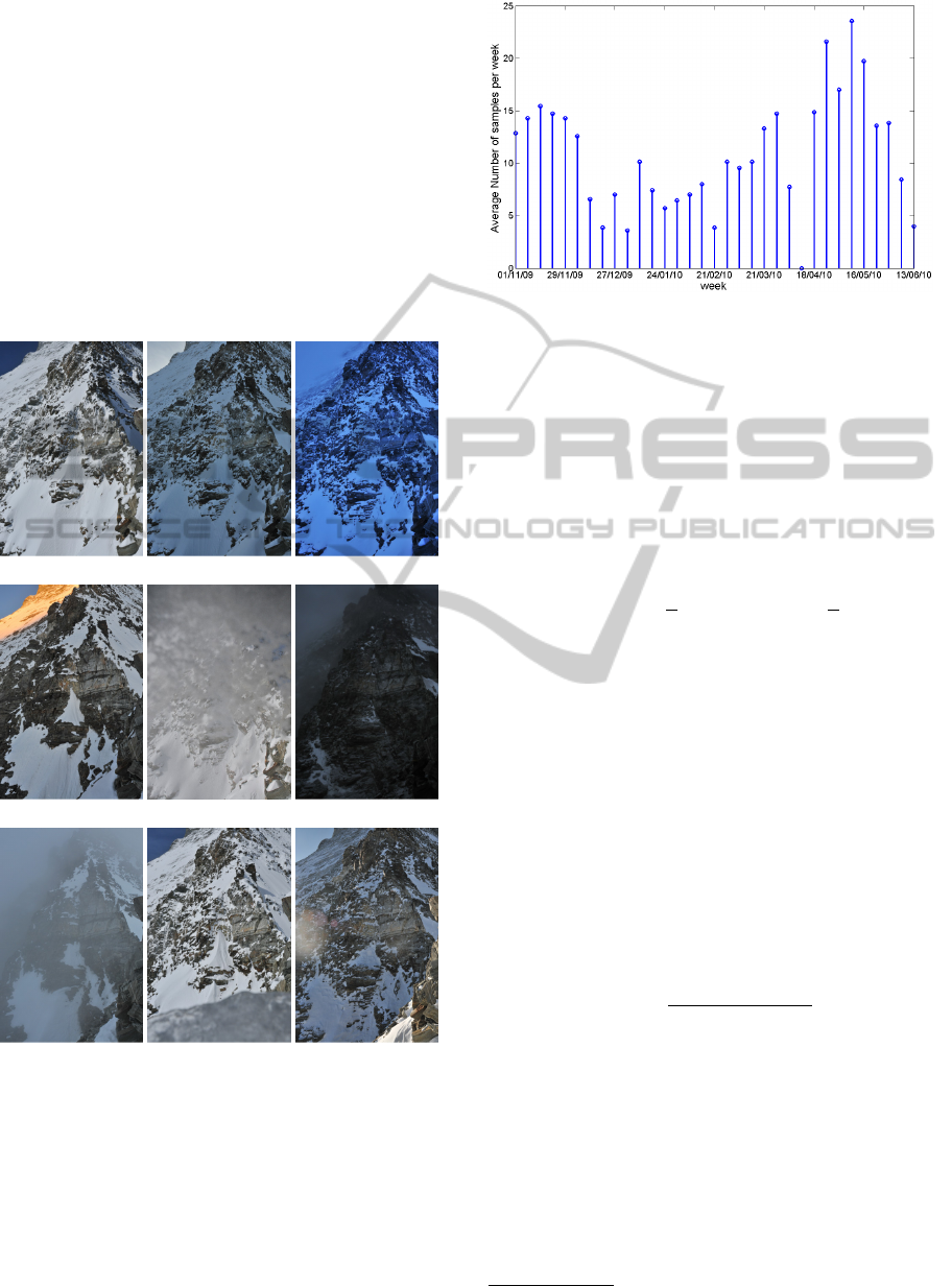
Keller et al., 2009b). Figure 1 shows typical images

present in the database. Ideally, the camera should

(a) Clear day (b) Overcast (c) Wrong WB

(d) Sunrise (e) Snowfall (f) Dark

(g) Fog (h) Ice on lens (i) Lens ﬂare

Figure 1: Images representing the variety of the image

database. All are in our manually labelled ground truth set.

take hourly captures, but since it is powered using

solar panels and there are long periods without sun-

shine, at times the camera cannot operate. In fact,

only around 2500 images are present in the database,

which is about 50% of the images that should have

been taken on an hourly basis. Figure 2 shows the av-

erage number of images per week. One can see the

Figure 2: Average number of samples per week.

big variations in the number of images taken. There

are even weeks where there is no image taken at all,

such as in the ﬁrst week of April 2010.

4.1 Splitting Up the Data

In the following, we denote L(m, n) the intensity value

of pixel (m, n) of an image L.

Images that are too

dark, such as the one in Figure 1(f), are not suited

for the GMM of color. We exclude all images whose

mean intensity value L is below 0.2, i.e. L < 0.2, and

refer to this reduced dataset as daytime images.

Using domain knowledge, we are able to identify

types of images in the dataset that systematically give

wrong snow cover estimations. Our classiﬁer used to

select the good (informative) images from all daylight

images is based on the following two observations:

• Blurry Images: Snow cover maps we obtain for

images that are blurry (i.e., because of fog, see

Figure 1(g)) are most often wrong. We apply a

Gaussian low-pass ﬁlter on L to get L

low

. The

high-frequency components of L are then simply

high

= L −L

low

. We deﬁne a sharpness index s

by the following ratio:

s =

∑

high

(m, n)|

∑

low

(m, n)|

. (7)

Since we want to drive our model using good im-

ages, it is less acceptable to have false-positives

than false-negatives. We manually tagged 250

good and 250 uninformative images, and then

set the threshold on s such that we have a false-

positive rate of less than 1%. Figure 3 shows the

histogram for the sharpness index computed for

the selected 250 good and 250 uninformative im-

ages. The green vertical line at s = 0.0289 indi-

z = L(m, n)

TemporallyConsistentSnowCoverEstimationfromNoisy,IrregularlySampledMeasurements

277

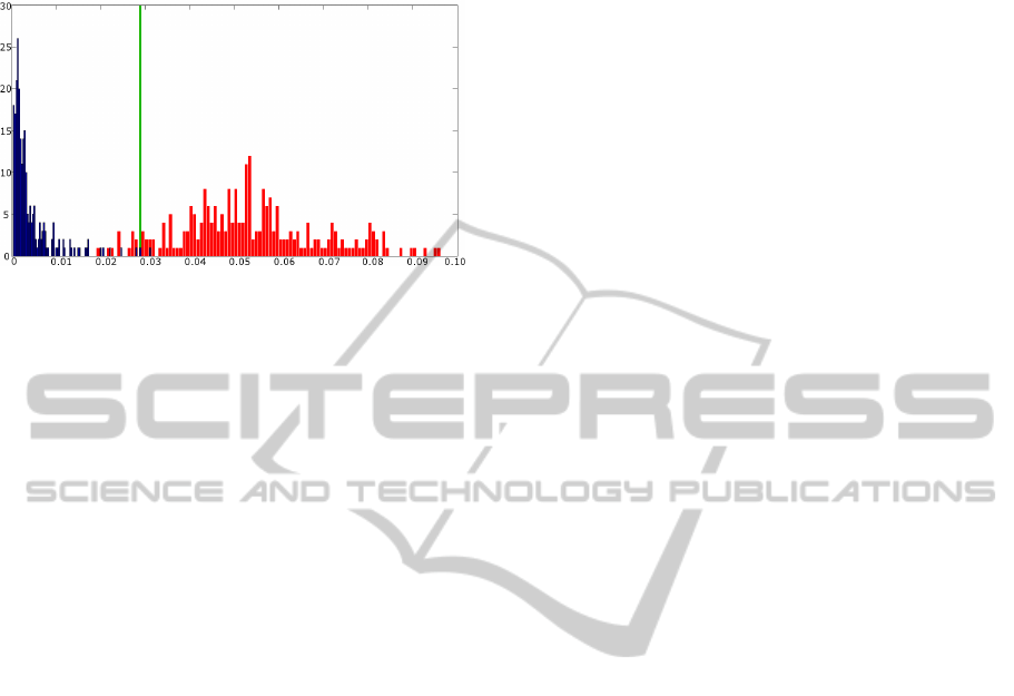
cates where the above condition was satisﬁed. We

therefore exclude all images where s < 0.0289.

Figure 3: Histogram of the sharpness indexes computed for

the 250 good (red) and the 250 uninformative (blue) im-

ages. The green vertical line shows the smallest value of

the sharpness index such that there are less than 1% false-

positives.

• Sunny Images: In images taken on a sunny day,

the rock in the middle casts a big shadow onto the

snow, as can be seen in Figure 1(a). This results

in the fact that the shadowed pixels are no longer

detected as snow. We found that these images can

be quite well excluded by imposing a threshold on

the minimum of the negative snow likelihoods:

min

−log p(z

= 1) < T

. (8)

In our case, T

= −5 allowed to best discriminate

between good and uninformative images.

After discarding the images labelled as uninformative

(728 dark, 766 blurry, 358 sunny images), we are left

with 659 good images. Note that 2396 of the 2491

images present in the image database were classiﬁed

correctly, giving an overall classiﬁcation correctness

of 96.2%. The false-positive rate on all images is

1.8%. It is worth noting that “foggy” and “sunny”

images could give more information about the scene

(e.g., cues for 3D structure), but this is left for future

work.

5 TEMPORAL CONSISTENCY

We achieve temporal consistency by formulating an

energy minimization problem, which involves the ini-

tial snow cover estimates computed in Section 3 as

well as a penalty term for different assignments. We

also tested weighted average and median ﬁltering for

comparison.

5.1 Markov Random Fields (MRF)

Traditional ﬁltering approaches such as (weighted)

average and median ﬁltering are not sensitive to the

data, they simply smooth it. We therefore used an

MRF, which have a data term and a prior term. In its

general form, an MRF can be written as follows:

p(z, x) =

∏

p(z

) ·

∏

j∈N(i)

p(x

, x

), (9)

where i indexes over all pixels in space and time, and

N(i) is the set of neighbors directly adjacent to pixel

i in space and time dimensions. Taking the log, the

products “simplify” to sums, and we get the following

global energy function we want to minimize:

−log p(z, x) =

∑

, x

) +

∑

j∈N(i)

, x

(10)

where the data term f

, x

) = −log p(z

) is the

negative log likelihood, computed using the GMM

of color (see Section 3). For the prior term, we use

a Potts Model f

, x

) = λ

i, j

−x

|, which can be

seen as a penalty for a change in snow-state in space

or time dimensions. The minimum of the global en-

ergy function in Equation (10) can be efﬁciently com-

puted using Graph Cuts (Boykov et al., 2001). With

i, j

we set how strong the bond between two neigh-

boring pixels i and j is, which controls the amount of

smoothing in the spatial domain and the number of

snow changes in the temporal domain.

Ideally, one would stack up all the informative images

present in the database and apply Graph Cuts on the

whole block to ﬁnd the best solution. With the aim of

reducing the memory requirements, we applied Graph

Cuts separately in the spatial and the temporal domain

by only connecting adjacent pixel neighbors in space

and time, respectively. We observed that in order to

get temporally smooth results, it is sufﬁcient to con-

nect each pixel with its neighbors in time, and to apply

Graph Cuts on those time vectors independently.

We denote the resulting image at time instant t

with penalty term λ as H

. For comparison, we im-

plemented two traditional ﬁltering approaches.

5.2 Weighted Average Filtering

The Gaussian ﬁltered snow cover map at time instant t

is computed as follows:

(m, n) =

∑

k=−r

∑

i=−r

∑

j=−r

i, j,k

·L

t+k

(m + i, n + j),

(11)

VISAPP2014-InternationalConferenceonComputerVisionTheoryandApplications

278

i, j,k

2πσ

√

2πσ

−



+ j



, (12)

where r

, r

∈ Z deﬁne the spatial and temporal ﬁlter

size, and σ

and σ

are chosen such that the Gaussian

weights approach zero for i = j = ±r

and k = ±r

respectively.

5.3 Median Filter

The median ﬁlter is known to be robust to outliers.

The median ﬁltered snow cover estimation map M

is computed as follows:

(m, n) = med{L

t−r

(m −r

, n −r

), ...,

t+r

(m + r

, n + r

)},

(13)

where med{·} denotes the median operator.

6 RESULTS AND DISCUSSION

6.1 Ground Truth

We created binary ground truth of 19 images by hand-

labelling pixels using GIMP (see Figure 4). They

(a) Input image (b) Snow pixels

labelled in GIMP

truth map

Figure 4: How the binary maps were created. We created

a new layer in GIMP, where all snow pixels of the input

image (a) were painted in red (b). Every red pixel was then

assigned a “1”, and the rest a “0”, which results in the binary

snow map shown in (c).

represent the variability of the image dataset, sam-

pled over the whole time span of the set. Examples

of images in the ground truth set are shown in Fig-

ure 1, as well as Figure 9. For images where parts

are obstructed, such as Figure 1(e), we used informa-

tion from the nearest unobstructed neighbors in time

to get as close as possible to the true amount of snow

coverage. We compare the ground truth on a pixel-

by-pixel basis with the resulting snow cover maps of

Figure 5: Dashed rectangles represent all images in the

database, “X” marks a ground truth image, ﬁlled rectangles

are computed snow cover estimates. Maps are compared

pixel-wise (orange rectangle). If the estimate for a ground

truth does not exist, we select the one closest in time (red

rectangle).

the different methods. As we exclude certain images,

it can happen that we do not have an estimate at the

time instant of the ground truth image (e.g., only 7 out

of the 19 ground truth images were labelled as good

images). In order to compute the classiﬁcation cor-

rectness, we thus took the snow cover map closest in

time (see Figure 5).

6.2 Finding the Best Parameters for

GMM of Color

Being a parametric model, the GMM has several pa-

rameters one can optimize. We tested several combi-

nations of number of mixture components, as well as

type of covariance matrix Σ (spherical and full). We

also transformed the images to the most relevant color

spaces before applying the GMM of color. We found

that the results were generally better using a spherical

covariance matrix. Figure 6 shows the accuracy ob-

tained for different combinations of number of mix-

ture components and color spaces using a spherical

covariance matrix.

Figure 6: Results for different color spaces and number of

mixture components, using a spherical covariance matrix.

We can see that with the exception of the Lch

color space, best results are always obtained for three

mixture components. When it comes to selecting the

color space, we can see that XYZ slightly outperforms

the standard sRGB color space, as well as the oppo-

TemporallyConsistentSnowCoverEstimationfromNoisy,IrregularlySampledMeasurements

279

nent color spaces we tested. The accuracy for HSV

and HSL is almost 10% lower than for the other color

spaces, so these two are not well suited for snow seg-

mentation.

6.3 Filtering Parameters

Our goal is to obtain an accurate, temporally con-

sistent estimation of snow coverage. There are dif-

ferent reasons why snow cover estimations based on

single images are inaccurate. As mentioned in Sec-

tion 4, quite a lot of the images are corrupted by

external factors, which inﬂuence the quality of our

snow classiﬁcation using a GMM of color: Shad-

ows cast on snow results in the fact that these regions

are wrongly classiﬁed as “not snow”, reﬂections of

the sunlight on (wet) stone makes those regions very

bright, and hence they are misclassiﬁed as “snow”

(see Figure 9(d)). Even more problematic is precipita-

tion on the lens, as well as foggy weather, which leads

to large parts of the image that are misclassiﬁed. To

a smaller extent, there might also be misclassiﬁcation

due to sensor noise. We investigated various combi-

nations of spatial and temporal ﬁlter lengths for both

the weighted average and the median ﬁlter, as well as

different weights for the MRF.

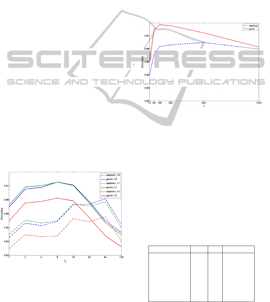
Median Filter. Since the median ﬁlter generally

gave better results than the weighted average ap-

proach, we show the accuracy obtained for various

combinations of spatial and temporal ﬁlter sizes for

the median ﬁlter (see Figure 7). Note that the tem-

poral half ﬁlter length r

was increased by factors of

Figure 7: Results for different combinations of spatial and

temporal ﬁlter sizes using median ﬁlter, for both the daytime

and the good image set.

The best results are obtained using only the good

images. We can see that the ﬁlter size can be reduced

by a factor of 8 as compared to the daytime images

(from 64 to 8), since there are fewer wrong snow esti-

mates. This allows the ﬁlter to faster adapt to changes.

We also see that the results drop by more than 1% for

a spatial ﬁlter size r

= 2 as compared to smaller ﬁl-

ter sizes. We found that r

= 1 resulted in slightly

more temporal consistent results, which is why we set

= 1.

MRF. As mentioned before, the MRF was only ap-

plied in the temporal domain because of computa-

tional complexity and memory requirements. Figure

8 shows the results for various weights λ:

Figure 8: Results for different weights using for the MRF,

for both the daytime and the good image set.

As with the median ﬁlter, the results are consis-

tently better when using only the good images. The

weight λ can be set lower, which results in better re-

activity to changes in snow coverage. This justiﬁes

the exclusion of uninformative images.

6.4 Comparison of the Methods

Table 1 summarizes the best results obtained for each

method on our ground truth set, both for all daytime

images, as well as for the good images only.

Table 1: Overall classiﬁcation correctness (C), standard de-

viation (σ), and reactivity to changes in snow coverage (R)

on 19 images, for the Gaussian Mixture Model (GMM),

weighted average (WA), median (Med), and Markov Ran-

dom Field (MRF), using the daytime or the good

†

images.

Method C σ R

GMM of color 83.3 8.7 immediate

WA 85.6 7.3 slow

Med 86.1 6.9 slow

MRF 86.5 6.6 fast

†

86.5 7.6 slow

Med

†

87.2 6.8 fast

MRF

†

87.9 6.1 very fast

VISAPP2014-InternationalConferenceonComputerVisionTheoryandApplications

280

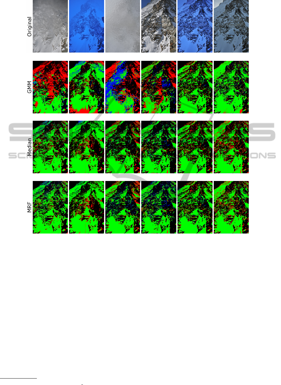
(a) 10.11.2009 (b) 09.05.2010 (c) 01.12.2009 (d) 15.02.2010 (e) 03.12.2009 (f) 02.03.2010

69.4% 83.1% 61.4% 77.9% 90.1% 89.6%

88.0% 89.4% 88.4% 90.9% 90.0% 85.5%

89.1% 90.1% 88.6% 89.4% 90.1% 86.9%

Figure 9: Comparison of the methods. Green are the true positives, blue the false positives, red the false negatives, and black

the true negatives. First row are the originals, second row the results of the GMM of color. Rows three and four show the

results obtained for the median ﬁltering approach M

1,8

and the MRF H

100

, respectively.

The reactivity to changes in snow coverage as well

as the temporal smoothness were subjectively evalu-

ated by watching a time lapse video. The videos can

be found on our web page

. One can see the trend that

the results are better for the good images, irrespective

of the method used to achieve temporal consistency.

Figure 9 shows results obtained on the good images.

Images (a)–(c) are examples where the temporal in-

formation can signiﬁcantly improve the classiﬁcation

accuracy, because the images are distorted. Image (d)

is interesting because it shows how the GMM of color

is fooled by shadows (upper right side), as well as

illuminated rock (center right part), which are both

misclassiﬁed. Again, one can see how the results im-

prove by incorporating information from neighboring

http://ivrg.epﬂ.ch/research/snow segmentation/

images in time. Images (e) and (f) both give reason-

able results using the GMM of color. In fact, using

temporal information slightly deteriorates the accu-

racy of the snow maps, because the snow coverage

is different in neighboring images. The MRF gives

slightly better results than the median ﬁlter approach,

because it is able to faster adapt.

Not only the classiﬁcation correctness is the high-

est for the MRF approach, but this method is also tem-

porally smooth and reacts very fast to changes in snow

coverage. This is due to the fact that the MRF is not

just a simple smoothing of the labels, as in the me-

dian ﬁlter, but in fact a data-sensitive and temporally

smooth labelling. This is a big advantage of the MRF

over the two basic ﬁltering approaches, as is exempli-

ﬁed in Figure 10, where two consecutive images of

TemporallyConsistentSnowCoverEstimationfromNoisy,IrregularlySampledMeasurements

281

Original L

1,8

100

Original L

t+1

1,8

t+1

100

Figure 10: Crop of two consecutive snow maps, before and

after a major snow fall. (a) and (d) are the originals, (b) and

(e) the median ﬁltered maps M

, and (c) and ( f ) the MRF

t+1

. The MRF almost completely reacts to the change in

snow coverage.

the database are shown.

The image at instant t (2. February 2010,

11.30am) is the last one taken just before the one at

t + 1 (3. February 2010, 2.26pm). A major snow fall

happened in-between, which explains the important

changes in snow coverage. Note how the median ﬁlter

approach is unable to adapt to the changes and under-

estimates the amount of snow coverage at time instant

t + 1, whereas the MRF approach is adapting almost

completely.

7 CONCLUSIONS AND FUTURE

WORK

We propose a technique for robust snow cover estima-

tion from time-lapse imagery. Since many of the im-

ages are uninformative, single image snow segmen-

tation using GMM of color is insufﬁcient to get tem-

porally consistent results. We use Markov Random

Fields (MRF) and formulate the temporal consistency

problem as an energy minimization, where we use a

penalty term to penalize neighboring pixels (spatially

and temporally) with different labels. Due to the na-

ture of the image data, the weight of the penalty term

has to be quite large in order to provide temporally

consistent results. The higher the weight, the less re-

active the model is to changes in snow coverage. Us-

ing domain-knowledge, we propose a classiﬁer to ex-

clude most of the uninformative images. Using only

the good images allows to relax the temporal con-

straints, making the model more reactive to changes.

The proposed model is both robust to outliers as well

as very reactive to changes in snow coverage.

Future work includes attempting the joint optimiza-

tion over space and time of Equation (10), and the

implementation of a snow deposition model, which

would be useful for long periods of uninformative

and/or missing images. This model could be used in-

stead of the zero-order hold we applied, resulting in

smoother transitions between two good images. An-

other interesting path to follow is to have different

models for different weather states, which could help

improve the initial snow cover estimations.

ACKNOWLEDGEMENTS

This work is in part supported by the National Com-

petence Center in Research on Mobile Information

and Communication Systems (NCCR-MICS), a cen-

ter supported by the Swiss National Science Founda-

tion under grant number 5005-67322.

REFERENCES

Blake, A., Rother, C., Brown, M., Perez, P., and Torr, P.

(2004). Interactive image segmentation using an adap-

tive GMMRF model. European Conference on Com-

puter Vision (ECCV), pages 428–441.

Boykov, Y., Veksler, O., and Zabih, R. (2001). Fast ap-

proximate energy minimization via graph cuts. IEEE

Transactions on Pattern Analysis and Machine Intel-

ligence, 23(11):1222–1239.

Breitenstein, M. D., Grabner, H., and Van Gool, L. (2009).

Hunting Nessie - Real-Time Abnormality Detection

from Webcams. IEEE International Conference on

Computer Vision (ICCV), pages 1243–1250.

Floros, G. and Leibe, B. (2012). Joint 2D-3D temporally

consistent semantic segmentation of street scenes.

IEEE Conference on Computer Vision and Pattern

Recognition (CVPR).

Hasler, A., Talzi, I., Beutel, J., Tschudin, C., and Gruber,

S. (2008). Wireless sensor networks in permafrost

research-concept, requirements, implementation and

challenges. Proceedings of the 9th International Con-

ference on Permafrost (NICOP).

Jacobs, N., Roman, N., and Pless, R. (2007). Consistent

temporal variations in many outdoor scenes. IEEE

Conference on Computer Vision and Pattern Recog-

nition (CVPR).

Keller, M., Beutel, J., and Thiele, L. (2009a). Demo

Abstract: MountainviewPrecision Image Sensing on

High-Alpine Locations. Adjunct Proceedings of the

6th European Workshop on Sensor Networks (EWSN),

pages 15–16.

Keller, M., Y

ucel, M., and Beutel, J. (2009b). High-

Resolution Imaging for Environmental Monitoring

Applications. Proc. International Snow Science Work-

shop, pages 197–201.

VISAPP2014-InternationalConferenceonComputerVisionTheoryandApplications

282

Khoshabeh, R., Chan, S. H., and Nguyen, T. Q. (2011).

Spatio-temporal consistency in video disparity estima-

tion. In IEEE International Conference on Acoustics,

Speech and Signal Processing (ICASSP), pages 885–

888.

MacQueen, J. (1967). Some methods for classiﬁcation and

analysis of multivariate observations. Proceedings of

the ﬁfth Berkeley symposium on Mathematical Statis-

tics and Probability, pages 281–297.

Nayar, S. and Narasimhan, S. (1999). Vision in bad

weather. IEEE International Conference on Computer

Vision (ICCV), pages 820–827.

TemporallyConsistentSnowCoverEstimationfromNoisy,IrregularlySampledMeasurements

283