
Statistical Models of Shape and Spatial Relation-application
to Hippocampus Segmentation
Saïd Ettaïeb
1
, Kamel Hamrouni
1
and Su Ruan
2
1
Université de Tunis El Manar, Ecole Nationale d'Ingénieurs de Tunis, Research Laboratory of Image,
Signal and Information Technology, Tunis, Tunisia
2
LITIS-Quantif, University of Rouen, Rouen, France
Keywords: Spatial Relations, Active Shape Model-ASM, Statistical a Priori Knowledge, MRI, Hippocampus.
Abstract: This paper presents a new method based both on Active Shape Model (ASM) and spatial distance model to
segment brain structures. It combines two types of a priori knowledge: the structure shapes and the distances
between them. This knowledge consists of shape and distance variability which are estimated during a
training step. Then, the obtained models are used to guide simultaneously the evolution of initial structure
shapes towards the target contours. The proposed models are applied to extract two hippocampal regions on
coronal MRI of the brain. The obtained results are encouraging and show the performance of the proposed
model.
1 INTRODUCTION
One of the main problems of medical images
segmentation is that they often present several
anatomical structures having no clear boudaries and
whose appearance is very similar. The automatic
separation of regions of interest is often a difficult
task. In particular, the use of techniques based only
on the low-level characteristics of the image is not
reliable, because the intensity of a pixel cannot give
certain information about its membership in a
structure. A promising way to remove ambiguity and
improve the performance of segmentation results is
to exploit high-level a priori knowledge, related to
the studied anatomical structures. Among this
knowledge, there are the spatial relations between
the structures in the same scene. These relations
represent structural knowledge for an image. They
are often more stable than the appearance
characteristics of the structures themselves.
Thus, they can be advantageously used to
improve the segmentation of medical images.
In this context, we propose to develop a new
model based on the Active Shape Model-ASM
(Cootes, 1995) and a spatial relation of distance. The
objective is to define a robust model capable to
segment two structures of interest simultaneously
using two types of a priori knowledge: the shape of
each structure and the distance between them. So,
the idea is to take advantage of statistical a priori
knowledge of shape and integrate a new knowledge
about the variability of spatial distance relation
between the structures to be segmented. This
knowledge is represented by a statistical distance
model estimated during a training step. The obtained
model will be then used to guide the evolution of
two initial shapes towards the target structures and
guarantee the preservation of the distance between
shapes in an authorized interval.
The proposed model is validated on a clinical
application, where the problem consists in
segmenting two structures of interest: two
hippocampal regions (left and right) on coronal MRI
of the brain.
This application represents a major interest in
clinical practice for early diagnosis of Alzheimer's
disease.
This paper is organized as follows. In Section 2,
we present spatial relations and their previous use in
medical images segmentation. Section 3 is devoted
to the integration of a statistical distance model to
guide the segmentation process. In Section 4, the
proposed model is applied to extract two
hippocampal regions on coronal MRI of the brain.
448
Ettaïeb S., Hamrouni K. and Ruan S..
Statistical Models of Shape and Spatial Relation-application to Hippocampus Segmentation.
DOI: 10.5220/0004658404480455
In Proceedings of the 9th International Conference on Computer Vision Theory and Applications (VISAPP-2014), pages 448-455
ISBN: 978-989-758-003-1
Copyright
c
2014 SCITEPRESS (Science and Technology Publications, Lda.)

2 SPATIAL RELATIONS
Spatial relations can be defined as the set of "facts"
that describe the location of objects in space. They
are mainly expressed by prepositions, which connect
several entities: "A is next to B", "A is near B", "A
is on the right of B", "A is inside B", "A is in front
of B "," A is behind B "," A is between B and C ",
etc. Some authors like [Freeman in 1975, Borillo in
1998] tried to define standard vocabularies in order
to describe the spatial relations. Generally, these
relations can be classified in three main categories,
considered as fundamental: the topological relations
used to describe the adjacency between structures
("is adjacent to", "crosses ", "is included"), the
distance relations representing the distance between
structures ("close", "far", "to a distance of ") and the
direction relations based on the six usual directions.
These relations represent interesting structural
information to model and interpret a scene. In the
medical field, the human body is a typical example
of structured scenes. Several books of anatomy
presented many linguistic descriptions involving
spatial relations between anatomical structures of the
body. It seems that the modeling and the use of these
relations are an interesting way to remove ambiguity
and constrain the segmentation procedures to be
more reliable.
Among the first remarkable work available on
this subject, we find that of Geraud (Geraud, 1998).
He proposed a sequential method of recognition of
brain structures, where every structure is recognized
thanks to the structural information resulted from the
previously recognized structures. This information is
generated from relations of distance and direction
defined with regard to the already segmented
structures. In the same context, Bloch and al
proposed, in (Bloch, 2003), a method where the
segmentation is performed from the beginning in a
zone of interest defined by the spatial relations. In
(Perchant, 2002), Perchant proposed a procedure for
recognition of brain structures based on the
matching of graphs: a graph derived from a
reference image manually segmented by an expert
and a graph of the image to be recognized. On the
graphs, the nodes are the structures of interest and
the arcs are the spatial relations between these
structures.
In the mentioned work, spatial relations are
mainly used in the step of recognition of anatomical
structures. The real segmentation is made with
classic methods. As part of his thesis work (Colliot,
2003), Colliot presented a particularly interesting
work, where spatial relations are used effectively in
the segmentation step. Relations such as direction,
distance and adjacency are represented by fuzzy sets
and integrated into the evolution equation of the
active contour (Kass, 1987) as an external force. For
the segmentation of a given structure, this force
attracts the curve towards the image areas where the
considered spatial relations are verified. Other recent
studies were also proposed (Hudelot, 2008,
Fouquier, 2010), where spatial relations are used
either in the stage of recognition or in the
segmentation step.
Our contribution is in this context and with the
same concept as the work proposed by Colliot and
Al. Indeed, we propose to model statistically the
spatial distance relation "A is at a distance of B" and
to use it directly in the segmentation step. This
relation will be expressed as a statistical distance
model and will be then integrated into the
segmentation procedure of ASM.
3 STATISTICAL MODEL
OF SHAPE AND SPATIAL
RELATION
The main idea is to combine the ASM with a priori
knowledge about the variation of a spatial distance
relation, in order to define a new statistical model of
shape and spatial relation.
The proposed model requires two main steps:
- A Training step, which aims to deduce from the
training set three elementary models: a statistical
shape model for every structure and a statistical
distance model which expresses the variation of
the distance between them.
- A segmentation step, based on the obtained models
to guide the simultaneous evolution of two initial
shapes towards the two target structures.
3.1 Training Step
This step consists in collecting at first a set of
samples of images reflecting the possible variations
of two structures to be segmented. Then, we extract,
from each image, the shape of each structure by
placing a sufficient number of landmarks on the
target contours. Considering that and are
respectively the number of landmarks required to
represent the details of the first and the second
structure and is the number of images in the
training set, each structure can be represented by a
matrix of points defined as follows:
StatisticalModelsofShapeandSpatialRelation-applicationtoHippocampusSegmentation
449

,
,
….
….
….
….
….
….
….
….
….
….
….
….
….
….
….
….
with
is the vector of points which models the
structure on the image.
,
are the
coordinates of the point placed in the image on
the contour of the structure. From these two
matrices, the shape model of each structure and the
corresponding distance model can be constructed.
3.1.1 Construction of Statistical Shape
Models
The construction of a statistical shape model is
described in detail in (Ghassan, 1998). Indeed, from
two obtained matrices of points, we can calculate the
mean shape relative to each structure:
∑
(1)
∑
(2)
After a step of shapes alignment and by applying the
PCA, we can also determine the modes and the
amplitudes of deformation of every shape. Each
structure can be then defined by a shape model that
describes its geometry and deformation modes.
These models can be respectively defined by:
(3)
(4)
with:
and
are respectively the matrices of the main
deformation modes of the first and the second
structure.
and
are two weight matrices which
represent respectively the projection of the shape
in the base
and the shape
in the base
.
3.1.2 Construction of the Statistical Distance
Model
The construction of the statistical distance model is
made at the same time as that of the shapes models.
It first consists in calculating the distances between
both structures of interest from the training images
and then trying to deduce a compact and precise
formulation, which describes the authorized
distances.
Given an image of the training set where both
structures of interest are modeled respectively by the
two following vectors:
,
,
,
,…,
,
,…,
,
,
,
,
,…,
,
,…,
,
M
x
,y
and M
x
,y
are any two points
of the first and the second structure. The Euclidean
distance between M
and M
is defined by:
,
(5)
If the Euclidean distance of each landmark of the
first structure with all points of the second one is
calculated, we can define a matrix of distances with
positive coefficients of rows and columns:
,
(6)
The elementary distance
between the two
structures of interest on an image is chosen as the
Euclidean distance between their two closest
landmarks:
,
,
min
(7)
Similarly, we can calculate the distances between
both structures of interest through all the images of
the training set. The result is a vector of
dimension:
,
,……,
,……,
(8)
The objective now is to deduce a compact
formulation that describes authorized distances.
Indeed, from the vector
, we can calculate the
following basic statistical parameters:
- the mean distance between two structures of
interest :
∑
(9)
- the variance which measures the dispersion of
elementary distances (
around the mean
distance:
∑
(10)
(The more the variance is high, the more the
variation of the distance between structures from an
image to another one is important).
- the standard deviation, which represents the mean
of all the elementary distances around the mean
distance:
(11)
VISAPP2014-InternationalConferenceonComputerVisionTheoryandApplications
450

Using these parameters, we can calculate the
confidence interval around the mean, which includes
a large percentage of the initial elementary
distances. Usually, the most adopted degree of
confidence is equal to 95.4%. This degree leads to a
confidence interval, limited as follows:
2,
2
(12)
This means that if we consider a new image to be
segmented, the distance between both structures of
interest belongs to the interval at 95.4%. (NB: An
increase of the degree of confidence leads to a
spreading of the confidence interval and thus a
decrease in precision). Finally, we can propose a
compact formulation of the distance between
structures defined as follows:
2φ
(13)
with φ is a real parameter in the interval
1,1
.
The equation 13 defines then the desired
statistical distance model. This model represents
thus a priori knowledge on the variation of distance
between structures. It can be effectively used in the
localization phase, to constrain the evolution of the
initial shapes. For that purpose, we should calculate
at each iteration the parameter φ as a function of the
current distance
(distance between the two shapes
in the current iteration). Equation14.
φ
2
(14)
There are then three possible cases:
I
f
φ ∈
1,1
Thenvaliddistance
I
f
φ 1←1
I
f
φ 1Thenφ ←1
(15)
In this way, we can require that the distance between
shapes will always be in the authorized interval. This
allows avoiding the divergence and the collision of
shapes during the evolution and increasing the
accuracy of results.
3.1.3 Integration of Distance Constraint
The integration of the distance constraint during the
evolution can be defined by the algorithm presented
in Table 1.
Table 1: Limitation by distance constraint.
: current distance, φ: real parameter,
:
shape1,
: shape2, , : real variables,
: mean
distance,:
If φ∈
1,1
Then valid distance
Else_if φ1Then #
2
2
/2
/2
Else #
2
2
/2
/2
End
End
3.2 Segmentation Guided by Shapes
Models and Distance Model
The segmentation phase consists in placing, first of
all, two initial shapes (mean shapes of two target
structures) on the image to be segmented: a
shape
, close to the first structure and a shape
,
close to the second structure. Then, every iteration is
divided into two basic steps:
- First, the initial two shapes evolve independently
of each other, according to the constraints imposed
by the corresponding shapes models.
The
evolution of shapes is based on the luminance
properties of the processed image. This provides
two intermediate shapes
and
.
- Then, we calculate the current distance
between
and
and we estimate the real parameterφ.
This allows applying the constraint imposed by the
distance model (equation 15) and thus producing
two new shapes with a valid distance between
them.
This process is repeated until no significant
changes are detected or the maximum number of
iterations is reached. Thus, segmentation takes into
account two essential information: the shape
constraints related to each structure and a global
constraint of distance between them. This
localization phase can be simulated by the algorithm
presented in Table 2.
StatisticalModelsofShapeandSpatialRelation-applicationtoHippocampusSegmentation
451

Table 2: Segmentation guided by shapes models and
distance model.
0
Initialization _ shape1 :
Initialization_ shape2 :
While (convergence==no and
_max_
1.
′
=evolution_shape1(
,
)
2.
′
=evolution_shape2(
,
)
3.
=distance (
′
,
′
)
4.
,
)= distance _limitation
(
,
′
,
′
,
2φ)
5. Convergence=compare (
,
)
&
,
))
6. i=i+1
End
4 APPLICATION
TO HIPPOCAMPUS
SEGMENTATION IN MRI
The hippocampus is a brain structure that is part of
the cortex. This is a pair structure, which appears in
an almost symmetrical way in each hemisphere. It is
involved in several neurological diseases including
Alzheimer's disease, which currently represents a
major problem of the public health. In clinical
practice, an early diagnosis of Alzheimer's disease is
based, necessarily, on the detection of atrophy of
hippocampal structures.
Many segmentation methods have been proposed
to contribute to the quantification of hippocampal
atrophy. Given the small size of this structure and
the imprecision of its limits, the proposed methods
are often based on a priori models (topology,
texture, relative position, etc.). These models are
derived from a statistical training set (Pizer, 2001
Pitiot, 2002, Yang, 2004) or an anatomical atlas
[Shen, 2011]. Pure deformable models have been
also used (Shen, 2002, Bailleul, 2007, Rajeesh,
2011). In (Babalola, 2008), the authors presented an
interesting qualitative and quantitative comparison
of four methods (Aljabar, 2007, Babalola, 2007
Patenaude, 2007, Murgasova, 2007) that were
applied to the segmentation of internal brain
structures on MRI, including the hippocampus.
The problems faced in these applications mostly
come from poor anatomical definition of the
hippocampus and the close similarity of its intensity
with the surrounding tissues intensities. The
isolation of hippocampal structures is often a
difficult task. They are generally treated among
other structures. In this work, we propose to
contribute to the segmentation of hippocampal
structures by relying on two types of a priori
knowledge: a priori on the shape of each part
separately (in each hemisphere) and a priori on the
distance between them.
4.1 Qualitative Results
The application of our model requires first the
construction of a training set. In this application, we
used 18 MRI brain volumes. From each volume, we
selected four T1-weighted coronal slices, where the
hippocampal structures are represented. We thus
obtained a set of 72 images of size 512*512 pixels.
50 images were used for the training and 22 images
were reserved for the tests. In the training step, 30
landmarks are placed on each image: 15 points to
extract the shape of the hippocampus in the right
hemisphere, and 15 points to extract it in the left
one.
The variability percentage of the initial data is
fixed to 95% and the length of the grey levels profile
in the training step is 7 pixels. As a result, we ended
up building a shape model for each part of the
hippocampus and a distance model, which models
the variation of the distance between them. The
obtained parameters of the model are shown in
Table 3.
Table 3: Parameters of shapes models and distance model.
hippocampus
(right part)
Hippocampus
(left part)
Shapes
models
7 principal
variation modes
6 principal
variation modes
Distance
model
Mean distance
62.26 ,
Standard deviation : 14.19
In the localization phase, the initializations used in
the various tests are calculated, each time, according
to the mean shapes obtained during the training. The
maximum number of iterations is fixed to 60 and the
length of the search profile is 19 pixels.
Figure 1 shows an example of the localization
result of the hippocampal structures, by presenting
the effect of the distance constraint in intermediate
iterations. Figure 2 shows the corresponding result
by ignoring the distance constraint (using the same
conditions).
The intermediate results in iteration 1 and
iteration 10 (Figure 1) show that the application of
the distance constraint helped to push positively the
shapes to the regions of interest. This explains the
remarkable difference between the accuracy of the
VISAPP2014-InternationalConferenceonComputerVisionTheoryandApplications
452
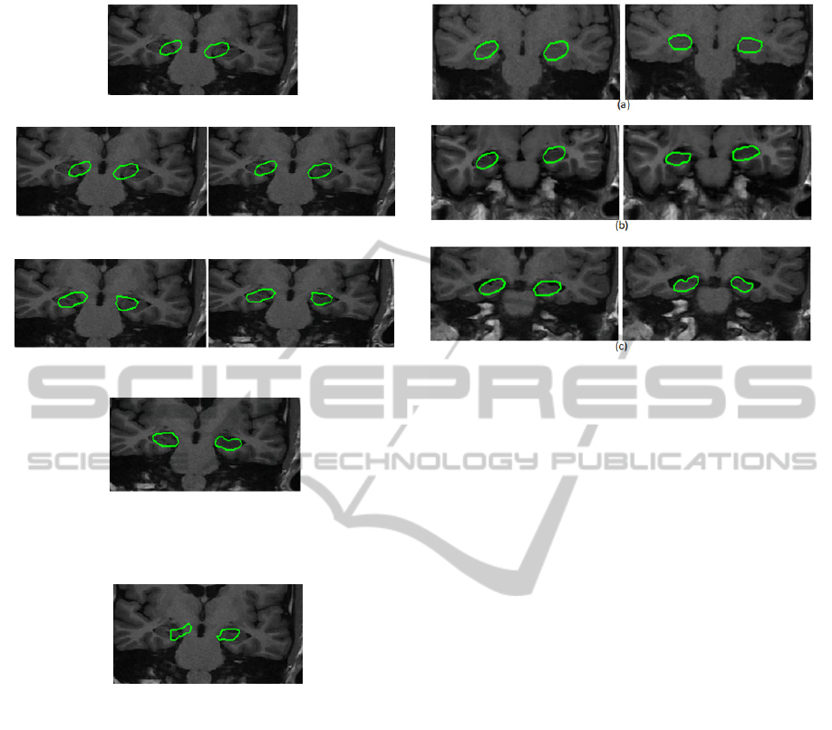
Figure 1: Result of the segmentation of the hippocampal
structures by ASMD
Figure 2: Result of the segmentation by ignoring the
distance constraint.
final result by ASMD (our contribution) and that
obtained by ignoring the distance constraint.
Figure 3 shows some segmentation results
obtained on patients with different stages of
hippocampal atrophy. We can notice that the initial
shapes succeeded in capturing the hippocampal
structures with different levels of atrophy. Thus,
qualitatively, we can conclude that the results
obtained by the proposed model for the
segmentation of the hippocampus on MRI slices are
satisfactory.
Figure 3: Examples of results obtained on patients with
different stages of hippocampal atrophy. The first column
shows the initializations and the second column shows the
corresponding results. (a) case of healthy patient (b) case
of patient with a mid-stage of atrophy (c) case of patient
with a late stage of atrophy.
4.2 Quantitative Results
For the quantitative evolution, first, ten slices of the
test database are selected and manually pre-
segmented in order to be used as references. This
ground truth is built with the help of an expert. Then
we decided to compare our contribution ASMD with
the ground truth, the original model of the ASM
(without distance constraint) and another method
proposed by Babalola and Al (Babalola, 2007). This
latter, abbreviated PAM, is a variant of Active
Appearance Model-AAM (Cootes, 1998) whose
texture model is based on perpendicular profiles in
the limits of the structure to be segmented and not
on all its shape. The results of this comparison are
presented in figure 4. It illustrates, by graph, the
distance of Hausdorff between every method
(ASMD, ASM and PAM) and the ground truth.
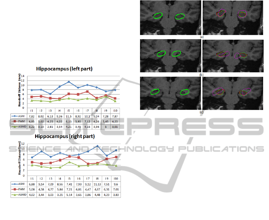
We can note that the Hausdorff distances found
by ASMD for both parts of the hippocampus, vary
from 2.81 (mm) to 5.14 (mm) with a global average
of 3.74 (mm). These measures are lower than those
found by the other two methods (ASM and PAM).
We also note that both methods PAM and ASM in
some cases give results close to the reference.
However, they generate in other cases very different
results even on the same slice. On the contrary, the
results of ASMD have some stability and coherence
between left and right part of almost all slices.
This is due to the fact that the segmentation of
Initialisation
Before limitation by distance
constraint
Before limitation by distance
constraint
After limitation by distance
constraint
After limitation by distance
constraint
Iteration 10 Iteration 1
Final localization result
StatisticalModelsofShapeandSpatialRelation-applicationtoHippocampusSegmentation
453
both hippocampal structures, with ASMD, is made
in a parallel and dependent way and is guided by
two constraints: the shape and the distance. These
results show the performance of the proposed model
and the benefit of the integrated distance constraint.
This additional constraint forced the initial curves to
evolve regularly according to an acceptable distance
and it thus channeled the evolution in the regions of
interest.
Figure 4: Results of the Hausdorff distance between the
three methods (ASMD, ASM and PAM) and the ground
truth.
In order to deduce the benefit of the integrated
distance constraint relatively to the initialization, we
made a comparison between the proposed ASMD
model and the original model ASM compared to the
ground truth. The comparison is performed on the
same image with the same propagation conditions
and by adopting different initializations. The results
are shown in Figure 5. We can notice on the column
2 a clear difference between the quality of results.
Indeed, for the three initializations, green curves
(results obtained with ASMD) are closest to the red
curves (reference segmentation). The second and the
third initializations (shown respectively in the figure
5.b and 5.c) are placed relatively far from
hippocampal structures. We see that, unlike the
green curves (ASMD results), the purple curves
(ASM results) fail to reach the regions of interest.
These results show that the used distance
constraint partially solved the known problem of
deformable models on initialization. It offers more
flexibility during initialization.
Figure 5: Comparison of results. The first column shows
the different initializations. The second column shows the
superposition of corresponding results: ASMD (green
curves), ASM (purple curves) and the manual
segmentation (red curves).
5 CONCLUSIONS
We presented an original segmentation model based
on the ASM and a spatial distance relation. It allows
the segmentation of two structures using two types
of a priori knowledge: the shape of each structure
and the distance between them. The proposed model
is validated on a clinical application, where the
problem is to segment two structures of interest: the
extraction of two hippocampal regions (left and
right) on coronal MRI of the brain. The obtained
results are encouraging and show well the
performance of the proposed model.
Although it showed its robustness and stability in
the majority of tests, the proposed model has some
limits and a number of perspectives that should be
mentioned. First, the model is designed to segment
two structures of interest, what limits the fields of its
use. In addition, the integrated distance constraint is
modeled by using the distances between the target
structures independently from their positions in the
image. Thus, theoretically and during the
localization, the distance between shapes may be
valid even if they are really far from the structures of
interest. This may produce false results.
Improvements in our model are then considered.
Indeed, it is possible to increase its reliability by
considering one of the two structures as a fixed
reference and to model the distance variation
according to this reference. This however requires a
VISAPP2014-InternationalConferenceonComputerVisionTheoryandApplications
454

prior segmentation of the structure that will be
considered as a reference. The proposed model can
easily be extended to segment several structures. It
means, for example, considering the simplest
structure to be segmented as reference and to
segment the others with regard to this reference.
REFERENCES
Cootes, T. F., Taylor, C. J., Cooper, D. H., and Graham J.,
1995. Active Shape Models - Their Training and
Application. Computer Vision and Image
Understanding, vol.61, pp38-59.
Freeman, J., 1975. The modeling of spatial relations.
Computer Graphic and image processing, Vol. 4, pp.
156-171.
Borillo, A., 1998. L’espace et son expression en français.
Ophrys, Paris.
Geraud, T., 1998. Segmentation des structures internes du
cerveau en imagerie par résonnance magnétique
tridimensionnelle. Thèse de Doctorat, Télécom paris.
Bloch, I., Géraud, T., and Maître, H., 2003. Representation
and fusion of heterogeneous fuzzy information in the
3d space for model-based structural recognition-
application to 3d brain imaging. Artificial Intelligence,
Vol. 148, pp. 141–175.
Perchant, A., and Bloch, I., 2002. Fuzzy Morphisms
between Graphs. Fuzzy Sets and Systems, Vol. 128, pp.
149–168.
Colliot, O, 2003. Représentation, évaluation et utilisation
de relations spatiales pour l’interprétation d’images.
Application à la reconnaissance de structures
anatomiques en imagerie médicale. Thèse de doctorat,
Telecom Paris.
Kass, M., Witikin, A., and Terzopoulos, D., 1987. Snakes:
Active contour models. International Journal of
Computer vision, vol.1, pp. 321-331.
Hudelot, C., Atif, J., and Bloch, I., 2008. Fuzzy Spatial
Relation Ontology for Image Interpretation. Fuzzy Sets
and Systems, 159:1929–1951.
Fouquier, G., 2010. Optimisation de séquences de
segmentation combinant modèle structurel et
focalisation de l’attention visuelle. Application à la
reconnaissance de structures cérébrales dans des
images 3D. Thèse de doctorat, Ecole Nationale
Supérieure des Télécommunications.
Ghassan, H., 1998. Active Shape Models - Part I:
Modelling Shape and Gray Level Variations.
Proceedings of the Swedish Symposium on Image
Analysis.
Pizer, S. M., Joshi, S., Thomas Fletcher, P., Styner, M.,
Tracton, G., and Chen, J. Z., 2001. Segmentation of
Single-Figure Object by Deformable M-reps. MICCAI,
vol.2208, pp.862-871.
Pitiot, A., Toga, A. W., and Thompson, P. M., 2002.
Adaptive Elastic Segmentation of Brain MRI via
Shape-Model-Guided Evolutionary programming.
IEEE TMI, vol.21, pp.910-923.
Yang, J., Staib, L. H., and Duncan, J. S., 2004. Neighbor-
Constrained Segmentation With Level Set Based 3-D
Deformable Models. IEEE TMI, vol.23, pp.940-948.
Shen, K., 2011. Automatic Segmentation and Shape
Analysis of Human Hippocampus in Alzheimer’s
Disease. Thèse de Doctorat, Université De Bourgogne.
Shen, D., Moffat, S., Resnick, S. M., and Davatzikos, C.,
2002. Measuring Size and Shape of the Hippocampus
in MR Images Using a Deformable Shape Model.
Neuroimage, Vol.15-2, pp.422-434.
Bailleul, J., Ruan, S., and Constans, J. M., 2007. Statistical
Shape Model-based Segmentation of brain MRI
Images. International Conference of the IEEE EMBS,
Lyon, France, 2007.
Rajeesh, J., Moni, R. S., and Palanikumar, S., 2001. A
versatile algorithm for the automatic segmentation of
hippocampus based on level set.
International Journal
of Biomedical Engineering and Technology.
Babalola, K. O., Patenaude, B., Aljabar, P. , Schnabel,
J., Kennedy, D., Crum, W., Smith, S., Cootes, T. F.,
Jenkinson, M., and Rueckert, D., 2008. Comparison
and Evaluation of Segmentation Techniques for
Subcortical Structures in Brain MRI. MICCAI.
Aljabar, P., Heckemann, R., Hammers, A., Hajnal, J., and
Rueckert, D., 2007. Classifier selection strategies for
label fusion using large atlas databases. MICCAI.
Babalola , K. O., Petrovic, V., Cootes, T. F., Taylor, J. C.,
Twining, J. C., Williams, T. G., and Mills, A., 2007.
Automated segmentation of the caudate nuclei using
active appearance models. In 3D Segmentation in the
clinic: A grand challenge. Workshop Proceedings,
MICCAI.
Patenaude, B., Smith, S., Kennedy, D., and Jenkinson, M.,
2007. Bayesian shape and appearance models.
Technical report TR07BP1, FMRIB Centre -
University of Oxford.
Murgasova, M., Dyet, L., Edwards, A. D., Rutherford, M.,
Hajnal, J., and Rueckert, D., 2007. Segmentation of
brain MRI in young children. Acad. Rad.
Cootes, T. F., Edwards, G. J., and Taylor, C. J., 1998.
Active appearance models. European Conference on
Computer Vision, pp 484–498.
StatisticalModelsofShapeandSpatialRelation-applicationtoHippocampusSegmentation
455
