
High Performance Particle Tracking Velocimetry for Fluidized Beds
Jouni Elfvengren, Jari Kolehmainen and Pentti Saarenrinne
Department of Engineering Design, Tampere University of Technology, Korkeakoulunkatu 6, Tampere, Finland
Keywords:
Particle Tracking Velocimetry, Fluidized Bed, Particle Sizing, GPU Computing.
Abstract:
Fluidized beds are used in wide variety of industrial applications. These applications range from energy
production to chemical industry. Particle tracking velocimetry (PTV) is an efficient way to study small scale
behavior inside fluidized beds. An accurate PTV algorithm has to be able to perform also in relatively dense
suspensions where particles may overlap and form clusters. PTV algorithms typically proceed from locating
the particles to tracking their motion. Typically the particle locating has been based on either profile matching
or image intensity thresholding. This study proposes a combined method that tries to take advantage of the
both methods to overcome difficulties associated with dense suspensions. The method was tested in a synthetic
case and in an experimental fluidized bed case. The synthetic tests showed a slight increase in error when the
number of particles increased, but the error level remained acceptable. Results obtained from the fluidized
bed were visually inspected. Visual inspection showed that most of the particles were tracked correctly, which
suggests that the proposed method performs well also in practice.
1 INTRODUCTION
In a fluidized bed, the upward air flow from the grate
(located at the bottom of the bed) causes sand and
other solid particles to behave in a more fluid-like
manner. Fluidized beds are used in many industrial
applications, such as fuel boilers and other multiphase
chemical reactors. Due to the complexity of the flow
inside a fluidized bed, most of the research in this field
is more or less dependent on experimental informa-
tion.
Particle Tracking Velocimetry (PTV), as the name
suggests, is a measurement method where individual
particles are tracked. The particles may be already
present in the flow, for instance in a fluidized bed,
or they are inserted into the flow as tracer particles.
The examined flow must be illuminated by a powerful
light source (typically a laser) to obtain high enough
frame rate to capture quickly moving particles within
the short exposure time of a high-speed camera. Dis-
placement vectors are obtained by tracking the move-
ment of particles between sequential frames. Since
the frame rate is known, the velocity can be obtained
from the displacement.
PTV has been used in a wide variety of applica-
tions ranging from laser machining (Viitanen et al.,
2012) to biomedical research (Smal et al., 2007). In
the fluidized bed research, PTV is effective analysis
method for low volume fraction flows, where the solid
suspension is not too dense. This type of flow condi-
tion typically exists in the upper parts of the fluidized
bed. One of the main advantages of PTV is that it can
be used to describe the very small scale behavior, such
as the solid phase turbulence associated to so called
granular temperature (Dijkhuizen et al., 2006).
PTV is typically based on either profile matching
based on cross correlations, see for instance (Marxen
et al., 2000), or thresholding image greyscale values,
as done by (Feng et al., 2007). While the thresholding
approach is effective when there are only few particles
present, and their profile is simple, it fails in dense
suspensions. On the other hand, the profile matching
yields in poor accuracy for particle center points if no
interpolation or distribution fitting is applied. Reli-
able sub-pixel accuracy is a crucial property in high
frame rate applications, where the consecutive dis-
placements are small.
In this study, the solid phase of the fluidized bed
consisted of small spherical glass particles. The trans-
parent glass particles tend to generate non-Gaussian
profiles to image plane when light is supplied from
behind the particles relative to camera. The parti-
cles can be observed from the images as dark rings
which have bright centers. Although the profile is
non-Gaussian in general, the profile of a dark ring can
be approximated as Gaussian. The described shadow
441
Elfvengren J., Kolehmainen J. and Saarenrinne P..
High Performance Particle Tracking Velocimetry for Fluidized Beds.
DOI: 10.5220/0004659404410449
In Proceedings of the 9th International Conference on Computer Vision Theory and Applications (VISAPP-2014), pages 441-449
ISBN: 978-989-758-009-3
Copyright
c
2014 SCITEPRESS (Science and Technology Publications, Lda.)

profile of a particle is relatively easy to detect, and the
bright center points increase the performance of PTV
in dense suspensions.
In this work, a combined approach based on both
thresholding and profile matching is proposed. The
goal is to formulate a credible PTV algorithm that
would have excellent sub-pixel accuracy, while be-
ing able to perform also in dense suspensions, where
some particles are inevitably overlapped. The latter
property is crucial in fluidized bed research, since the
particles tend to form clusters, where they are very
close to each other. The performance of the pro-
posed method is improved by parallel computing on a
Graphics Processing Unit (GPU).
2 EXPERIMENTAL SETUP
The experimental setup of this study consists of a
nearly 2-dimensional fluidized bed, a diode laser and
a high-speed camera. A schematic illustration of the
experimental setup is shown in Figure 1. The flu-
idized bed is 6mm thick, and 100mm wide. It was
operated with inlet pressure of 0.8bar. The high speed
camera was placed in front of the bed. The bed was il-
luminated from behind by Cavitar HF diode laser with
wavelength of 810nm. The laser beam was expanded
with Cavitar micro optics. An optical bandbass filter
was also used to reduce random noise. The bandpass
filter was designed for the mean value of 810nm with
the bandwidth of ±10nm. Pressurized air was sup-
plied to an expansion zone beneath the bed and blown
to the fluidized bed via four grate nozzles. Before en-
tering the grate, air flow passes a humidifier, which
was used to decrease static electricity. Static electric-
ity can cause unwanted clustering and particle stick-
ing to the walls of the fluidized bed.
Particles tracked from digital images are typically
small tracer particles designed to follow closely the
motions of the examined flow. These tracer particles
range from < 1 to 30µm in diameter in gas flows ac-
cording to (Melling, 1997). However, in the exper-
imental case presented in this paper, the interest is
aimed at tracking the motion of substantially larger
spherical glass particles with the nominal diameter of
200µm. Most of these particles are clearly visible,
but some may be a bit out of focus, even though max-
imum possible depth of field (DOF) is achieved by
minimizing the size of the camera aperture while en-
suring sufficient exposure. Problems in detecting sin-
gle particles arise when multiple particles are packed
in clusters. Particles in a cluster can be only momen-
tarily joined together while moving in different direc-
tions at different velocities. They can also be bonded
together by surface forces and move as a group, which
is less usual based on the experimental data.
In general, an adequately high frame rate should
be chosen when recording very fast particle mo-
tions. The frame rate of the camera was thus set to
1500fps, and the focal ratio to f /12. These settings
kept the displacements of particles between consecu-
tive frames relatively small, while allowing sufficient
DOF as explained in the previous section. It should
be noted that when a coherent laser, such as Nd-YAG
laser, is used, setting the focal ratio too high can cause
unwanted total reflections from the diffuser. However,
the laser used in this study was not of the coherent
type, and the mentioned problem does not occur.
Optical fibre
Fluidized bed
Diffuser
Bandpass filter
Camera
Figure 1: Schematic picture of the measurement setup.
3 PTV ALGORITHM
3.1 Profile Matching Algorithm
When particle suspension is illuminated from behind,
there is usually a bright spot in the middle of the parti-
cle. The mid area between the boundary and the cen-
ter of the particle has typically the smallest intensity.
The detailed profile could be computed from the Mie
scattering theory (Bohren and Huffman, 1983). How-
ever, camera causes Gaussian blur to the profile an-
ticipated by the Mie theory. In addition, the sensor
voltage of the camera cell and light intensity might
not be linear. Therefore, in this study a more direct
approach is taken.
A particle image is thought to consist of a torus of
dark points with a diameter of d. Camera then sees a
shadow of each of these points. If the lowest intensity
of the particle is denoted by b, and the bright back-
ground intensity by w then the particle profile at point
x can be given by superposition
J(x) = w(1 − φ(x)) + bφ(x), (1)
where φ(x) is a profile function.
The profile function for the above mentioned torus
with Gaussian blur is given by
φ(x) =
Z
kyk=d
N(x|y,Σ)dy, (2)
VISAPP2014-InternationalConferenceonComputerVisionTheoryandApplications
442

where N(·|y,Σ) denotes the density function of a 2D
normal distribution with mean value y, and covariance
matrix Σ. In this study, the covariance matrix had a
diagonal structure.
The algorithm proceeds by looping over all the
points in an image. From each point y a neighbor-
hood of that point I
y
(x), also referred as the mask,
is compared to the profile computed by Equation (1).
The background intensity of the Equation (1) is cho-
sen prior any computations. The lower intensity value
b is estimated as the average color on a circle of ra-
dius d around the point y. The likelihood of point y
being the center of a particle is estimated as
f (y) =
Z
kJ(x) − I
y
(x)k
2
N(x|0,Σ
I
)dx, (3)
where Σ
I
is covariance matrix of the mask. The co-
variance matrix is used to increase the value of inte-
rior points over the boundary points, and is a common
approach when computing image correlations.
The mask was chosen as a square, with size of
12 × 12 pixels. A circular or ellipsoidal mask could
also be interesting, but a square mask was used due to
its simplicity. In Figure 2 an example particle and a
suitable mask for profile matching has been plotted.
Figure 2: Example particle (left) and suitable profile match-
ing mask (right).
Since the f values computed by Equation (3) are
independent on other f values, they can be com-
puted quite efficiently by a Graphics Processing Unit
(GPU). In the study, it was found out that most of the
time was spend in transferring the image to the GPU
memory from the Random Access Memory (RAM).
The bright particle centers were recognized from
the f values by searching local minimums. Since
the background is not completely homogenous due
to auto interference of the laser, there is typically a
large number of local minimums in the background.
However, the local minimums appearing in the back-
ground are typically larger by a magnitude than the
actual particles, and therefore are relatively ease to
distinguish from the actual particles.
The downside of the above described method is
that it is very sensitive to diameter value d. This
can cause multiple recognitions inside a single par-
ticle and some systematic errors, where the algorithm
places the center of particle systematically too near
the boundary of the particle. To remedy this problem
a clustering method can be used to connect too-near
recognitions.
3.2 Thresholding Method
In order to identify particles from a greyscale image,
it must be first decided whether a pixel of the image
contains information about a particle or not. In this
process, a binary image with ones representing the in-
formative particle regions and zeros representing the
non-informative background region is generated.
The most common binarization method is proba-
bly the single threshold binarization. In this method,
a single threshold value is selected and the binary im-
age is computed based on whether a pixel is above
or below the selected threshold value. Although
this method is simple and fast to execute, it requires
clearly separable particle greyscale values from the
background greyscale values. Even though the signal
to noise ratio (SNR) in the images would be sufficient,
this method lacks the ability to take account the non-
uniform illumination conditions typically present in
experimental setups.
In this paper, a correction of inhomogeneous illu-
mination is combined with the single threshold bina-
rization, leading to an efficient and reliable binariza-
tion method.
3.2.1 Correction of Inhomogeneous Illumination
In experimental setups, the inhomogeneous illumi-
nation conditions can be caused by several factors.
For example, the amount of illumination decreases to-
wards the light direction due to absorption and scat-
tering from the measured particles and the fluid, when
a laser light sheet is passed from one side to the cam-
era’s field of view. Also possible reflections from the
solid structures cause problems when using the sin-
gle threshold method. In the experimental setup pre-
sented in this paper, the uneven background illumi-
nation profile is caused by the diverging optics of the
back laser. The unevenness can be observed from the
decreasing greyscale values towards image edges.
The inhomogeneous illumination conditions can
be easily corrected if it is possible to obtain images
where the illumination conditions are otherwise sim-
ilar to the experimental setup but no particles are
present (J
¨
ahne, 2004). These images are usually
called as reference or background images. In order to
reduce the effect of random noise in the background
images, it is recommeded to compute pixelwise av-
erages across a reasonable set of background images.
HighPerformanceParticleTrackingVelocimetryforFluidizedBeds
443
The inhomogeneous illumination is corrected by di-
viding every pixel of the image G by the correspond-
ing pixel of the average background image R
C
mn
= c
G
mn
R
mn
, (4)
where scalar c is used to scale the grey values of the
corrected image. The scaling factor c was selected
as 100 in this work. Values of the corrected image C
can be thus considered as percentage of the image G
greyscale value to the background image R greyscale
value. Notice that the corrected image C is stored as
double precicion data type instead of the original im-
age’s 8-bit unsigned integers. An example of a ran-
dom particle image corrected by the average back-
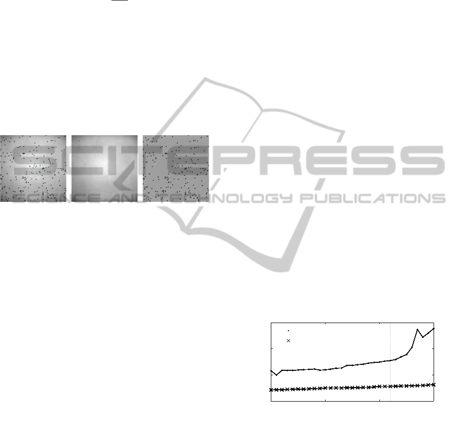
ground image is given in Figure 3.
Figure 3: Particle image, average background image and
illumination corrected particle image.
3.2.2 Single threshold Binarization
After the correction of inhomogeneous illumination,
it is possible to use the single threshold binarization
method with outstanding results compared to the non-
corrected images. The single threshold binarization
for corrected images is defined as logical operation
B
mn
=
1, if C
mn
≤ C
th
0, if C
mn
> C
th
,
(5)
where C
th
is the optimum threshold value.
While the correction of inhomogeneous illumina-
tion enables the usage of the single threshold binariza-
tion, it still leaves us the problem of selecting an opti-
mal threshold value. Basically the thresholded pixels
should contain as much information about the parti-
cle as possible, but false particles stepping out of the
background should not occur. On the one hand, when
decreasing the threshold value (in the case of dark
particles), some boundary pixels are left outside the
thresholded region. In this case some information of
the particle has been lost and the shape of the thresh-
olded boundary starts to have an effect on the particle
center point computation, leading to increased pixel
locking effect as shown by (Feng et al., 2007). On the
other hand, when increasing the threshold value (in
the case of dark particles) beyond the optimum value,
false particles start to arise from the background. The
size of the false particles range from 1 pixel to several
pixels, and the size increases as the threshold value
increases.
It is possible to search the optimum threshold
value by comparing the total amount of found par-
ticles at different threshold values from an extensive
sample of corrected particle images. If the minimum
size of the measured particles is clearly larger than the
size of the small false particles, containing only some
pixels, it is practical to remove all particles below a
selected minimum size in pixels (see Section 3.3.3).
It should be noted that also some incomplete parti-
cles located at the image edges are thus considered as
small particles. In the case of dark particles, the max-
imum threshold value, with which the total amount
of found particles remains at fairly constant level, is
selected as an optimum threshold. As pointed out by
(Feng et al., 2007), it should be also checked from a
sub pixel map that the pixel locking effect does not
occur at the selected threshold value.
The optimum threshold is determined experimen-
tally using every twentieth frame of the recorded data.
As can be seen from Figure 4, the amount of all
found particles begins to rise notably after the thresh-
old value 72, which is thus selected as the optimum
value. Interestingly, the amount of selected particles
remains very stable even when the total amount of
found particles starts a rapid rise. This is because the
small particles below a selected minimum size are re-
moved from the total amount of found particles lead-
ing to the number of selected particles. The observed
stability in the amount of selected particles is a highly
desirable feature of the algorithm.
50 60 70 80
8800
9000
9200
9400
threshold value
number of particles
← C
th
= 72
all particles
selected particles
Figure 4: Amount of all particles and selected particles as
function of threshold value.
A sub pixel map of particle locations in the opti-
mum threshold selection is presented in Figure 5. The
sample size of the corrected particle images was the
same as in the optimum threshold determination. No
visible pixel locking pattern (Feng et al., 2007) can be
observed, so the selected optimum threshold value is
adequate. In general, when the particle average size is
quite large (as in the experimental case), pixel locking
occurs in a smaller degree than in the case of particles
containing only some pixels.
VISAPP2014-InternationalConferenceonComputerVisionTheoryandApplications
444

0 0.5 1
0
0.5
1
Figure 5: Subpixel image for particle center point locations
at optimum threshold value.
3.3 Particle Indexing
In this work, the thresholding method is combined
with the profile matching method. The particle index-
ing is thus performed in two steps. In the first step,
thresholded particle regions in the binary image are
indexed by tracking their outer boundaries. In the sec-
ond step, particle clusters are separated based on the
center points recognized by the profile matching al-
gorithm. Each pixel of a particle cluster is re-indexed
using the criteria of closest distance to a center point.
After these steps, every pixel of every thresholded
particle region is given an index that determines the
particle in which it belongs to.
A major advantage in combining the profile
matching method with the thresholding method is the
sub pixel accuracy obtained by the calculation of the
particle center points from thresholded and indexed
pixels as explained in Section 3.4. Additionally, the
separation of particles from particle clusters increases
significantly the reliability of the identified particles
in comparison to plain thresholding method.
3.3.1 Thresholded Particle Region Indexing
The thresholded particle regions are indexed by track-
ing their outer boundaries using the Freeman chain
code of eight directions, explained by (J
¨
ahne, 2004).
In this algorithm, the binary image is scanned line by
line and when a binary value one (that is not yet in-
dexed) is found, the outer boundary binary ones are
tracked in clockwise direction using 8 possible neigh-
bor directions. In this work, all pixels inside the ob-
tained closed boundary are indexed by a number that
defines the particle. Even though there may be some
binary zero pixels inside the closed boundary (typi-
cally the bright spot in the middle of the particle), the
corresponding pixels of the corrected image C proba-
bly contain in some extent useful information and can
be thus considered as a part of the particle region.
3.3.2 Particle Cluster Separation
It is possible that an indexed particle region contains
multiple particles. The recognized particle center
points calculated with the profile matching algorithm
are used here to separate single particles from particle
clusters. If the indexed particle region contains more
than one center point, the pixels inside are separated
into re-indexed regions based on their closest distance
to a center point. When particles are not too over-
lapped and the center points are correctly recognized,
this method usually leads to well-separated particles.
The presented particle separation process com-
bines the advantages of the thresholding method and
the profile matching method. The thresholded particle
regions are considered to contain reliable information
of the particles being measured. By checking that a
center point recognized by the profile matching algo-
rithm is inside a thresholded region, it is ensured that
no false particle center point matches arising from the
background, are considered as actual particles. If the
profile matching algorithm has failed to recognize a
center point inside an indexed particle region, it is as-
sumed that the thresholded region is correct and con-
tains a single particle.
When particles are partially overlapped, some pix-
els evidently belong to both particles, but are straight-
forwardly divided to different particles using the pre-
sented separation method. This clearly leads to some
error in the calculation of the particle center point in
Section 3.4. In cases where particles are so over-
lapped that only one or no center point at all is rec-
ognized by the profile matching method, some error
also occurs in the calculation of the center point of the
overlapped particle cluster. The magnitude of these
errors can be examined by testing the method using
synthetic particle data.
3.3.3 Removing Small Particles
Even with the optimal threshold value some small
false particles can still occasionally arise from the
background. To ensure that no false particles are con-
sidered as real particles, all particles below a selected
minimum size in pixels are removed. Evidently, the
particle minimum size should be notably smaller than
the minimum size of the measured particles. The par-
ticle minimum size should be selected with care, be-
cause also some incomplete particles are inevitably
removed from the image edges. In this paper, approx-
imately 20% of the average size of the measured par-
ticles is used as the particle minimum size.
HighPerformanceParticleTrackingVelocimetryforFluidizedBeds
445

3.4 Particle Center Point Computation
The center point position of a particle is determined
by the greyscale value weighted position of pixels
X =
∑
i
X
i
(C
i
−C
base
)
∑
i
(C
i
−C
base
)
, (6)
where i represents the pixels belonging to an indexed
particle, X
i
is the pixel center point location vector,
C
i
is the corrected greyscale value of a pixel of the
particle i and C
base
is the base line value.
It has been shown by (Feng et al., 2007) that se-
lecting C
base
= C
th
minimizes the total error in the sub
pixel accuracy caused by the pixel locking effect as-
sociated with the pedestal part of the intensity that re-
mains below the threshold value. Also in this work,
the base line value equal to the optimum threshold
value is selected.
3.5 Particle Tracking
Several particle tracking algorithms have been devel-
oped for tracking the motion of single particles from
digital images. Although promising results have been
obtained using many of these methods, the authors de-
cided to demonstrate the performance of a relaxation
based tracking method. In this work, the original re-
laxation method (ORX), summarized by (Ohmi and
Li, 2000) and originally developed by (Barnard and
Thompson, 1980), is selected for tracking the parti-
cles. The implementation of the original relaxation
method used in this work follows closely to the one
presented by (Ohmi and Li, 2000). The new relax-
ation method introduced by (Ohmi and Li, 2000) was
recently further improved by (Jia et al., 2013). For the
sake of simplicity, the additional relaxation parame-
ters and other improvements to the original relaxation
method, discussed by (Ohmi and Li, 2000) and (Jia
et al., 2013) among other authors, are not studied in
this work. The original relaxation algorithm is eas-
ily expandable to include the latest improvements on
demand.
The relaxation methods calculate particle match-
ing probabilities iteratively until the probabilities
have converged to nearly constant levels. During
these iterations, the probability of a correct matching
particle is increased close to one. A major advantage
of the relaxation methods is the no-match probabil-
ity formulated in the relaxation algorithm, which re-
duces clearly the amount of false matching particles
compared to other particle tracking methods. A useful
feature is also the ability to define the search radiuses
R
s
, R
n
and R
c
(Ohmi and Li, 2000) to suitable values
depending on the examined case in order to achieve
high quality tracking results. In general, the relax-
ation methods work well in complicated flows and
dense particle regions in comparison to other meth-
ods (Jia et al., 2013), which suggest that these meth-
ods are applicable to the turbulent two-phase flow of
the fluidized bed examined in this article.
4 SYNTHETIC IMAGES
In this work, an artificial particle grayscale distribu-
tion is used to generate synthetic particles that re-
semble the particle profile observed in the actual im-
ages. The artificial greyscale distribution is defined as
a twin normal distribution expanded into two dimen-
sions by the equation
z(x,y) ∝ N(r(x,y))|µ,σ) + N(r(x,y))| − µ, σ), (7)
where
r(x, y) =
q
(x − x
0
)
2
+ (y − y
0
)
2
(8)
is the radius from the center point of the distribution
(x
0
,y
0
) to any specific point (x,y). The normal dis-
tribution N parameters were selected as µ = 2.6 and
σ = 1.7 and the distribution values z(x, y) were mul-
tiplied by an appropriate scaling constant c
s
to make
the greyscale values computed from the given distri-
bution similar to measured greyscale intensity profile.
Accurate values in every pixel of the synthetic image
were obtained by numerically evaluating the double
integral
G
p,mn
= c
s
Z
m+0.5
m−0.5
Z
n+0.5
n−0.5
z(x,y)dxdy (9)
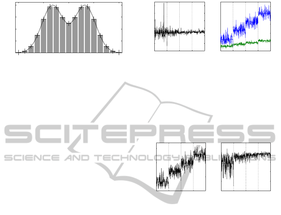
using a 9-point Gauss quadrature rule. The result-
ing center line profile of a synthetic particle G
p
with
center point placed at origin (X
0
,Y
0
) = (0,0) is pre-
sented in Figure 6. Notice the slight difference be-
tween the values integrated over every center line
pixel presented with bars and the values of the dis-
tribution function multiplied with c
s
and marked with
plus signs.
The synthetic particle images are generated by
randomly spreading a selected amount of the distri-
bution center points (x
0
,y
0
) into an image area of
1024 × 1024 pixels. Particles are then integrated one
by one from the distribution values using Equation
(9). When combining overlapped particles to a sin-
gle synthetic image, the maximum greyscale value in
the corresponding pixels is selected. In reality, the
scattering light does not behave this way, but this is
a reasonable simplification since the actual scattering
profile is not modeled.
VISAPP2014-InternationalConferenceonComputerVisionTheoryandApplications
446
−8 −4 0 4 8
0
20
40
60
80
position (pixels)
grayscale value
Figure 6: Cross-sectional greyscale profile of synthetic par-
ticle.
The standard deviation of the background
greyscale values is estimated based on an image,
where no particles are present, corrected by Equation
(1). The mean of the normal distribution in the syn-
thetic background images is selected as µ = 100 and
the standard deviation is approximated as σ = 1.5. As
a result, a synthetic particle image including the back-
ground random noise is generated by subtracting the
synthetic particle image from the background image.
5 RESULTS
5.1 Generic Test
The errors encountered in particle center point calcu-
lation can be divided into two different groups. This
is achieved by computing the nearest computed center
point for every synthetic center point. If the amount
of synthetic center points connected to a single com-
puted center point is more than one, the synthetic
center point is considered to belong to multi-match
group. Otherwise it belongs to single-match group.
Obviously the sum of synthetic single-match particles
and synthetic multi-match particles equals the total
number of synthetic particles in a single frame.
The overall error in the synthetic test is computed
for each frame as the average of all distances between
a synthetic center point location and the closest com-
puted center point location. The average overall error
increases at nearly linear rate from 0.13 pixels (250
particles) to 0.42 pixels (1000 particles) as Figure 7
indicates. In Figures 7 and 8 there are 250, 500, 750
and 1000 synthetic particles in the frames 1-100, 101-
200, 201-300 and 301-400, respectively. The aver-
age value for every set of 100 frames is plotted as a
straight line to these figures.
In Figure 8 the effect of multi-match particles to
the overall error is compared. The increase of the
overall error is mostly caused by the synthetic center
points that are connected to multiple computed cen-
0 100 200 300 400
0
1
2
3
4
5
6
frame
error (pixels)
↓ multi−match
0 100 200 300 400
0
0.1
0.2
0.3
0.4
0.5
frame
error (pixels)
overall ↓
↓ single−match
Figure 7: Multi-match, single-match and overall error in
synthetic test.
ter points. The average effect of multi-match parti-
cles to the overall error increases as the total amount
of particles increases. Although the average error of
multi-match particles remains at almost constant level
around 2.45 pixels as Figure 7 indicates, the effect to
total error increases due to the increasing ratio of mul-
tiple matching particles presented in Figure 8.
0 100 200 300 400
0
5
10
15
frame
ratio to all particles (%)
multi−match ↓
0 100 200 300 400
0
20
40
60
80
100
frame
effect to overall error (%)
↓ multi−match
Figure 8: Ratio of multi-match particles to all synthetic par-
ticles. Effect of multi-match particles to overall error in syn-
thetic test.
The average error of single-match particles in-
creases as the amount of particles increases as can
be seen from Figure 7. Although the ratio of single-
match particles to all synthetic particles decreases
as Figure 8 conversely indicates, the average error
of single-match particles increases from 0.05 to 0.11
pixels. This is probably caused by the increased prob-
ability of neighboring particles, which inevitably re-
duces the sub-pixel accuracy as the thresholded pixels
of particle clusters are divided to separate particles.
5.2 Experimental Test
Figure 9 shows the selected amount of particles af-
ter thresholding, particle cluster separation and re-
moval of small particles. The selected amount of par-
ticles shows a high fluctuation because also the actual
amount of particles varies with a large amplitude in
the measurement area of the highly turbulent upper
part of the fluidized bed. However, the amount of se-
lected particles in sequential frames shows only mod-
erate fluctuations, which means that the amount of
HighPerformanceParticleTrackingVelocimetryforFluidizedBeds
447
computed particles in sequential frames is quite con-
tinuous, as it should. No unexpected outliers are ob-
served, which proves the robustness of the algorithm.
The amount of separated particles from the thresh-
olded particle regions is also presented in Figure 9. As
expected, the amount of separated particles increases
notably when the total amount of particles increases
and more particles become close to each other.
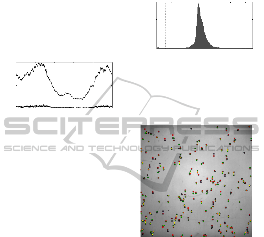
300 600 900 1200 1500
0
50
100
150
200
frame
number of particles
↓ selected
↓ separated
Figure 9: Selected amount of particles and separated
amount of particles from particle clusters.
The sub-pixel image for all computed center
points in every frame of the experimental test shows
no signs of pixel locking. This implies that the
computed center points matching a single particle
are within excellent sub-pixel accuracy (Feng et al.,
2007). As the synthetic test demonstrates, the ac-
curacy drops to pixel scale in cases where multiple
actual particles computed as one particle. However,
the degreased accuracy in the case of particle clusters
is at some degree diminished at the particle tracking
stage when suitable matching particles are not found
between sequential frames.
The particle size distribution is plotted as a his-
togram in Figure 10. The distribution contains a sin-
gle peak at the particle size of 141 pixels and has a
mean value of approximately 150 pixels. The num-
ber of particles is thus slightly more concentrated on
the right-hand side from the peak value. The reason
for this is probably that the algorithm is not able to
separate all particle clusters to single particles. If the
particles are somewhat normally distributed around
the nominal value, the measured particle size distribu-
tion should also resemble this distribution. The non-
separated particle clusters evidently shift the balance
towards larger size particles.
In Figure 11 a vector field computed from frames
319-320 is presented. The particle tracking is com-
puted by the original relaxation method (Ohmi and
Li, 2000). Parameters used in the experimental test
are R
s
= 28 for sequential radius (sequential frames),
R
n
= 90 for neighbor radius (first frame) and R
c
= 20
for parallel motion radius (sequential frames). The
selected value for parallel motion radius allows some
clearly erroneous displacement vectors. On the other
0 50 100 150 200 250 300
0
2000
4000
6000
particle size (pixels)
number of particles
← min size
Figure 10: Particle size histogram in experimental test. Par-
ticles below minimum size are removed.
hand, decreasing this value will cancel out many
good matching particles in sequential frames. In gen-
eral, when applied to highly turbulent flow where the
motion of single particles is chaotic, this parameter
should have clearly higher value than in flows where
the particle random motion is considerably smaller.
Figure 11: Sample vector field. Green equals initial and red
final computed center point locations.
The sequential radius of the particle tracking al-
gorithm is selected based on the observed particle
motion between two sequential frames. It should be
pointed out, that displacements exceeding this value
are not considered as possible matching particles. The
selection of the neighbor radius R
n
proves out to be
quite tricky, because the particle density varies highly
in different locations of a single frame and in different
frames of the experimental test. This problem is rarer
in tracer particle experiments, where the density of the
seeding particles remains typically at constant level.
As a solution to this problem, the authors propose in-
creasing the radius R
n
, until an adequate number of
neighbor particles are inside the perimeter. However,
in the experimental test of this work, the neighbor ra-
dius is simply set to a high enough value to include
some neighbor particles also in dilute regions.
VISAPP2014-InternationalConferenceonComputerVisionTheoryandApplications
448

6 CONCLUSIONS
The proposed method was tested in a synthetic test
case with computer generated random data, and with
a cold model fluidized bed. The synthetic test case
allowed one to inspect the behavior of the PTV al-
gorithm with varying number of particles. From the
synthetic test cases one can conclude that there are
two major sources of error, namely error caused by
finite sub pixel accuracy, and error caused by inabil-
ity to detect the particle. Both errors increased when
the number of particles was increased. However, the
latter error type became quickly dominant.
In statistical studies, usually the number of detec-
tions is not of main concern, but rather the credibil-
ity of the detections. As shown in the synthetic test
case results, sub pixel accuracy showed only slight
increase with the increase of particles. On the other
hand, most PTV based studies in fluidized beds are of
the statistical type. Thus the proposed method is well
suited for the fluidized bed research, or other simi-
lar problems, where particles exist in relatively dense
suspensions.
The proposed method was also tested in a cold-
model of a fluidized bed. Since the real displacements
are not known the data was only visually inspected.
Visual inspections showed that the method most of the
time able to detect particles, but failed occasionally to
detect all of the particles from clusters. On the other
hand, number of false positives (particle detections on
the background) was very small, which is especially
important in statistical studies.
Structure of the algorithm is easy to parallelize,
as particles interact with each other in very limited
way on the detection phase. The particle tracking al-
gorithm uses information of the neighboring particles,
which is difficult to parallelize, but is computationally
much less expensive than the detection phase. Profile
matching algorithm used in this study does assume
that the particle profiles are independent of the neigh-
boring particles. While this assumption is the key for
computational efficiency, it limits the maximum par-
ticle density. Future developments in this field are
likely to include interacting particles models, for fur-
ther improvements in accessible particle density.
ACKNOWLEDGEMENTS
This work has been done as a part of Online FB-CFD
project funded by TEKES. The authors would like to
thank S. Kallio and J. Peltola for helpful discussions
regarding the topic. In addition, authors would like
to thank Cavitar Ltd. for supplying lasers and optics.
As a source of useful information about multiphase
flows, the authors also wish to thank COST FP-1005
project for cooperation.
REFERENCES
Barnard, S. and Thompson, W. (1980). Disparity analysis
of images. IEEE Transactions on Pattern Analysis and
Machine Intelligence, 2:333–340.
Bohren, C. and Huffman, D. (1983). Absorption and Scat-
tering of Light by Small Particles. John Wiley and
Sons, New York, 1st edition.
Dijkhuizen, W., Bokkers, G. A., Deen, N. G., van Sint An-
naland, M., and Kuipers, J. A. M. (2006). Extension of
piv for measuring granular temperature field in dense
fluidized beds. American Insitute of Chemical Engi-
neering, 53:108–118.
Feng, Y., Goree, J., and Liu, B. (2007). Accurate particle
position measurement from images. Review of Scien-
tific Instruments, 78.
J
¨
ahne, B. (2004). Practical Handbook on Image Processing
for Scientific and Technical Applications. CRC Press,
Boca Raton, 2nd edition.
Jia, P., Wang, Y., and Zhang, Y. (2013). Improvement in
the independence of relaxation method-based particle
tracking velocimetry. Measurement Science and Tech-
nology, 24:055301 (13pp).
Marxen, M., Sullivan, P. E., Loewen, M. R., and Jahne, B.
(2000). Comparison of gaussian particle center es-
imators and the achievable measurement density for
particle tracking velocimetry. Experiments in Fluids,
29:145–153.
Melling, A. (1997). Tracer particles and seeding for par-
ticle image velocimetry. Measurement Science and
Technology, 8:1406–1416.
Ohmi, K. and Li, H. (2000). Particle-tracking velocimetry
with new algorithms. Measurement Science Technol-
ogy, 11:603–616.
Smal, I., Niessen, W., and Meijering, E. (2007). Advanced
particle fltering for multiple object tracking in dy-
namic fuorescence microscopy images. Biomedical
Imaging: From Nano to Macro, 4:1048–1051.
Viitanen, T., Kolehmainen, J., Okamoto, Y., and Piche, R.
(2012). Spatter tracking in laser machining. Proceed-
ings of 8th International Symbosium on Visual Com-
puting, pages 626–635.
HighPerformanceParticleTrackingVelocimetryforFluidizedBeds
449
