Tetrachromatic Metamerism

A Discrete, Mathematical Characterization

Alfredo Restrepo Palacios

Laboratorio de Se

nales, Dept. Ing. El

ectrica y Electr

onica, Universidad de los Andes,

Carrera 1 No. 18A-70; of. ML-427, Bogot

a 111711, Colombia

Keywords:

Metamerism, Tetrachromacy.

Abstract:

Two light beams that are seen as of having the same colour but that have different spectra are said to be

metameric. The colour of a light beam is based on the reading of severel photodetectors with different spectral

responses and metamerism results when a set of photodetectors is unable to resolve two spectra. The spectra

are then said to be metameric. We are interested in exploring the concept of metamerism in the tetrachromatic

case. Applications are in computer vision, computational photography and satellite imaginery, for example.

1 INTRODUCTION

Two light spectra are said to be metameric when the

corresponding lights look of the same colour. For ex-

ample, a spectral (i.e. of energy at a unique wave-

length) yellow light beam and an appropriate com-

bination of spectral beam lights, green and red. We

stress the point that it is pairs of spectra, and not pairs

of colors, that are metameric.

We explore the concept of metamerism in the

tetrachromatic case, mainly from a mathematical

viewpoint. Applications are in computer vision, non-

human biological vision, computational photography

and satellite imaginery, for example.

Given four photodectectors with spectral sensitiv-

ity curves w(λ), x(λ), y(λ), and z(λ), and the spec-

trum s(λ) of a light beam that falls on the surface

of each, the corresponding responses are given by

s(λ)w(λ), c

s(λ)x(λ), c

s(λ)y(λ)

and c

s(λ)z(λ). The integrals measure the area

below the spectrum curve (i.e. the radiant energy)

as ”seen through” each of the sensitivity curves. In

a sense, the sensitivity curves aperture sample the

spectrum. In such a tetrachromatic a vision system

two spectra giving rise to the same responses c

, c

and c

will be undistinguishble by the photode-

tectors and will be said to be metameric. The point

c = [c

] ∈ R

will be called a colour point;

In our case, we are old-world, fruguivore, trichromatic

primates and most of us have exactly three types of pho-

topigment in the main receptor layer of our retinae, but

many animals are tetrachromatic.

here, R denotes the set of the real numbers.

Thus, in going from s(λ) to c = [c

], you

take four aperture samples of s and metamerism re-

sults when the photodetectors are unable to resolve

two spectra. This is unavoidable if you consider that

a set of four photoreceptors linearly

maps the graph

curve of each spectrum function s : [λ

min

,λ

max

] →

[0,∞) into a point on the ”16-tant

” R

that we de-

note also as [+, +, +, +]:= {[t

] : t

≥ 0} of R

Figure 1: The rectangle is meant to be the domain space of

a linear transformation; the point at the center is the origin

of the space. The light green line is meant to be the kernel

of the transformation, the green lines are cosets and the red

line is the orthogonal complement of the kernel.

The fact that the irradiance of the light beam is non-

linearly contracted to a bounded luminance is being over-

looked here; nevertheless, regarding the hue, things are

pretty much linear..

Analogously to the cuadrants of the plane and the oc-

tants of 3-space.

Restrepo Palacios A..

Tetrachromatic Metamerism - A Discrete, Mathematical Characterization.

DOI: 10.5220/0004660200400047

In Proceedings of the 9th International Conference on Computer Vision Theory and Applications (VISAPP-2014), pages 40-47

ISBN: 978-989-758-003-1

 2014 SCITEPRESS (Science and Technology Publications, Lda.)

In order to use the machinery of linear spaces

with the transformation s 7→ c, we must allow both

spectra and color points to take on negative values as

well. The resulting sets of spectra R

[λ

min

,λ

max

]

and of

colours R

are now linear spaces and will be called

sets of virtual spectra and of virtual colours, respec-

tively. When a virtual spectrum is nonnegative we

say that is is realizable and, likewise, when the com-

ponents of a colour are nonnegative, we say that it is

a realizable colour.

The kernel of the transformation R

[λ

min

,λ

max

]

→

that maps s 7→ c, is the set of spectra that are

mapped to the colour point [0, 0, 0, 0], called here

black. The spectra in each corresponding coset of

spectra are mapped to the same (colour) point on R

;

this is the main idea behind a mathematization of the

phenomenon of metamerism. See Figure 1.

In our digital, technical world, magnitudes are

made discrete; a camera aperture-samples the spec-

trum of the light at each of many small spatial re-

gions or pixels. In addition to this, we assume that

such sampling is done over an already sampled spec-

trum, sampled at a much more ﬁner scale, e.g. ev-

ery 10 nm, or so. Thus, the interval set of wave-

lengths [λ

min

,λ

max

] ⊂ R is converted to a ﬁnite se-

quence {λ

= λ

min

, λ

, ... λ

= λ

max

} of wave-

lengths, and the transformation from spectra to colors

is now of the form R

→ R

, considerably simpler

and yet a good approximate model. Integrals become

dot products, i.e. c

= w.s =

∑

, c

= x.s =

∑

= y.s =

∑

and c

= z.s =

∑

Most mammals are dichromatic

and it has been

argued that the L photopigment evolved in old-world

monkeys as it resulted advantageous in the appraisal

of the ripeness of fruits when seen from the distance;

or, since male dichromacy is common in such pri-

mates, that it evolved providing females with health

cues regarding potential mates. In biological vi-

sion, tetrachromacy is found in ﬁsh, birds, reptiles

and in many invertebrates; the mantis shrimp is 12-

chromatic and sees in the range from 300 nm to 700

nm. In satellite imaginery, the bands may be many but

you may restrict to R, G, B plus either NIR or UV. In

both cases, the bands include some amount of overlap

but are mostly disjoint; unlike the case of a recently

developed detector for photography that, in addition

to the usual R, G and B pixels of a Bayer, array sen-

sor, it includes unﬁltered (other than by the glass of

the lens of the camera and the package of the sensor)

”panchromatic” pixels.

Spectral lights are perceived as more saturated

Most mammals have cones S (short wavelengths) and

M (medium wavelengths) but no cone L (large wave-

lengths). See (Jevbratt, 2013).

than more wide-band lights; thus, the spectral yellow

might appear a bit more saturated, than the yellow that

results from the mixture of green and red. In what

we call hue metamerism, luminance differences of the

light beams can be considered immaterial, as well as

the saturation, up to a degree. Two colors may have

the same hue but different luminance and different

chromatic saturation; correspondingly, a relaxed type

of metamerism may be also exploited in computer vi-

sion systems; differences in luminance may be due to

differences in illumination intensity and differences in

saturation may be due to atmospheric conditions but

not to different spectral reﬂectances of surfaces. In

this line, it is useful to consider a hypercube of pho-

todetector responses and identify sets of constant hue

or chromatic triangles, in it (Restrepo, 2013b), (Re-

strepo, 2013a).

Figure 2: Satellite RGB image and processed NIR-RGB im-

age. From (Restrepo, 2013b).

TetrachromaticMetamerism-ADiscrete,MathematicalCharacterization

2 TETRACHROMATIC

METAMERISM

Let w, x, y and z be four linearly independent, N-

vectors of samples of the spectral responses, at a set

of wavelengths λ

,...λ

, of four photodetectors; also,

let the (corresponding samples of the) light spectrum

be given by s. Denote the ”colour” response of the

photodetector set by c = [c

]. Assume then

that the response to a light beam falling on four such,

nearly placed, photodetectors is given by













=: Ms



















... w

... x

... y

... z



















This provides a linear transformation R

→ R

s 7→ r, that reduces the dimensionality from N to 4. M

has full rank and its entries are nonnegative and, typi-

cally, positive. Thus, for a nonnegative s, c is nonneg-

ative: c ∈ R

. The kernel K of this transformation

is given by the set of vectors k for which

Mk =













k =













Thus, K, the set of the metameric blacks, is the

space of vectors orthogonal to (each element of) the

subspace L := span{w,x,y,z} = {aM : a ∈ R

which is isomorphic to R

. Also, any two spectra

s and

s such that

s −

s ∈ L

⊥

= K, produce

the same colour response c = [c

]. L has

dimension 4 and L

⊥

has dimension N − 4; also,

: R

→ R

is invertible. K contains ”spec-

tra” (we might call them virtual spectra) that are

neither nonnegative nor nonpositive

. The cosets

s + K := {s + k : s ∈ R

,k ∈ K} provide a partition

of R

. In a decomposition s = f + k, f ∈ L, k ∈ K,

which is unique, f is called a fundamental metamer

and k is called a metameric black. The spectra in the

coset f + K are said to be metameric and are mapped

by M to the same colour point c ∈ R

; only the

nonnegative spectra in such coset are realizable, the

remaining are merely virtual.

The spectra in R

that are nonnegative are those in the

wedge or ”2

-tant” [+, +, ... +]:= R

N+

2.1 A Basis for K

Calling the colour point [0, 0, 0, 0] black, then K

is the set of spectra that ”evoke” the colour black;

call them metameric blacks. Since the components

of M are nonnegative, the only nonnegative spec-

trum that is a metameric black is the 0 spectrum; all

other metameric black spectra include both positive

and negative components.

Cohen’s method (Cohen and Kappauf, 1982),

based on CIE data, consists of ﬁnding f as f =

(MM

)

−1

M]s and then writting k = s − f.

We derive a basis for K of narrow-band spectra in

a 4-step process where 4 triangular, sparse matrices of

row vectors of local support are derived. In the ﬁrst

matrix

A you have a basis for the orthogonal comple-

ment of span{w}, in the second one

A, a basis for the

orthogonal complement of span{w, x}, then, in

A, a

basis for span{w,x,y}

⊥

and ﬁnally, in

A, a basis for

span{w,x,y,z}

⊥

. We assume that the components of

w, x, y and z, are positive so that the matrix

A below

is computable and also that each of the matrices

A and

A, as deﬁned below, are computable.

Let

A be the N × (N − 1) matrix with i

row of

the form [0, ..., 0, 1, −w

i+1

,0,...,0]; thus,

M has a

diagonal of 1’s. Clearly, each row of

A is orthogonal

to w and, since linearly independent, they provide a

basis for span{w}

⊥

Let each row of

A result from linearly combining

each pair of consecutive rows of from

A. In this way,

each row is still orthogonal span{w}

⊥

and, by using

appropriate weights in the combination, you can make

it also orthogonal to span{x}

⊥

. In fact, let the i

row

of the N × (N − 2) matrix

A be given by

[0,...,0,1,m

i,i+1

+ β

i+1,i+1

,β

i+1,1+2

,0,...,0]

where the m’s are the components of

A, and

= −

i,i+1

i+1

i+1,i+1

i+1

i+1,i+2

i+2

;

again, the diagonal of

A is a diagonal of 1’s. Like-

wise, by making sure a certain linear combination of

each two consecutive rows in

A is orthogonal to y,

you get the N × (N − 3)-matrix

A with i

row of the

form

[0,...,0,1,m

i,i+1

+ βm

i+1,i+1

i,i+2

+βm

i+1,i+2

,βm

i+1,i+3

,0,...,0]

where the m’s are now the components of

A and

= −

i+1

i,i+1

i+2

i,i+2

i+1

i+1,i+1

i+2

i+1,i+2

i+3

i+1,i+3

The diagonal of

A is a diagonal of ones. Finally, a

linear combination of each two consecutive rows in

A that is orthogonal to z, provides the N × (N − 4)-

matrix

A with i

row

[0,...,0,1,m

i,i+1

+ βm

i+1,i+1

i,i+2

+βm

i+1,i+2

i,i+3

+ βm

i+1,i+3

,βm

i+1,1+4

,0,

...,0],

where the m’s are now the components of M

and

VISAPP2014-InternationalConferenceonComputerVisionTheoryandApplications

= −

i+1

i,i+1

i+2

i,i+2

i+3

i,i+3

i+1

i+1,i+1

i+2

i+1,i+2

i+3

i+1,i+3

i+4

i+1,i+4

See Fig. 6. Let the rows of the N × (N − 4)-matrix

B :=

A denote this resulting base for the kernel K of

Note that the rows in each of these matrices

are linearly independent due to their localized

support. The rows in

A have support of length

2, those in

A have support of length 3, those

A have support of length 4 and those in the

basis B of L

⊥

= K have support of length 5. The

existence of β in each case is not so surprising due

to this localization; that is, for example, it is not

too difﬁcult to ﬁnd constants α

and β

so that

(α[1,−w

,0] + β[0,1,−w

]).[x

] =

[α,−αw

+ β, −βw

].[x

] = αx

(−αw

+ β)x

− (βw

= 0; letting α = 1,

you only need x

− w

+ β(x

− w

) = 0,

i. e., x

. In fact, when

computing

A, each β

can be also expressed as

= −

−

i+1

−

i+1

i+2

. Similar formulas of β can be

derived for the remaining cases of

A and

The addition of a scaled element of the so-

obtained basis for K is the addition of a metameric

black that alters the spectrum in a very narrow re-

gion of it producing a new metamer. Large peaks in a

base element of K may indicate indicate insensitivity

to certain wavelengths.

2.2 Sets of Metameric Spectra

The set of spectra R

is partitioned into cosets of

the form K + s, s ∈ R

. To each colour point c =

[w, x, y,z]

in the hypercube, there corresponds the

coset S

of dimension N-4, of spectra (not necessarily

realizable as physical spectra) that are mapped by the

matrix

M =













to such colour point. To ﬁnd S

, you ﬁnd a spectrum

vector s for which Ms = c and then write S

= K + s.

To ﬁnd one such s, choose a 4x4 matrix N given by

four columns of M, say the i

, j

columns:

N =













We assume that N is invertible; in fact we choose one

such matrix N having highest absolute determinant so

that the computation of its inverse is more accurate.

Regarding the possible values of the absolute value of

the determinant, there are





= 1.282.975 choices of

i, j,k, l to consider. Once one such matrix is chosen,

put t = N

−1

c and

s = [0, ...t

,0...t

,0,...t

,0,...]

s is not necessarily in L, i.e. it is not necessarily a

fundamental metamer; also, t may have negative com-

ponents; in such case, a spectrum s that is nonzero

only at positions i, j, k,l and produces colour c, is not

physically realizable. Only the nonnegative spectral

photoreceptor vectors in K + s are of realizable. It is

possible that a realizable colour not be the image of a

realizable spectrum.

If you are designing a tetrachromatic imaging

system and do not want spectra

s and

s to be

metameric, at least one of the pairs w.

s and w.

s, or

s and x.

s, or y.

s and y.

s, or z.

s and z.

s should

be different, in particular,

s −

s should be in L and

must not be in K; i.e.

s −

s ∈ L − K.

3 A CASE EXAMPLE:

RGB+PANCHROMATIC

Besides satellites, a source of tetrachromatic images

is computational photography. TrueSense Imaging

inc. markets a digital image sensor that, in addition

to R, G, and B pixels of a Bayer pattern, it includes

as well panchromatic pixels

in a pattern as shown in

Fig. 3. The proportions are 1/4 of green pixels, 1/8 of

red pixels, 1/8 of blue pixels and 1/2 panchromatic

pixels. Even though the photosensitive transducers

respond well into the UV, the microlens blocks wave-

lengths below 350 nm. The sensor responds in the

infrared but the response is negligible above 1050 nm.

The pattern of the color ﬁlter array is

Figure 3: Pattern in the array of the sensor Truesense Imag-

ing KAI-01150: P B P G; B P G P; P G P R; G P R P.

Pixels that are covered by the microlens but that other-

wise do not receive ﬁltered light.

TetrachromaticMetamerism-ADiscrete,MathematicalCharacterization

For our purposes, we do not need interpolate the

data in the pattern array that give rise to the image

shown at the top in Figure 4; instead, we downsample

each 4 × 4 pixel block to a tetrachromatic pixel, by

averaging the pixels in each band in the block. Thus,

even though the original image is 1152 × 2044, the

image we work with is only 287 × 510 pixels. Also,

the bands we use are w = P, x = R, y = G and z = B.

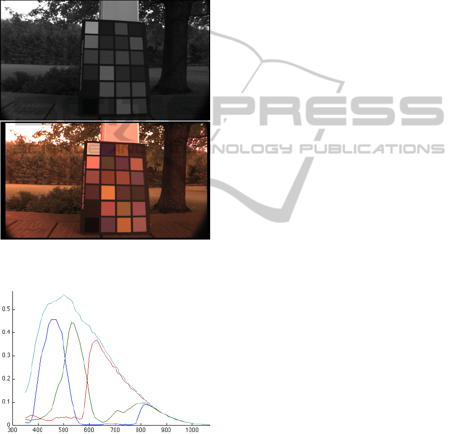
Figure 4: Outdoors, 16-bit, RGBP image of a Macbeth

chart; courtesy of Amy Enge. Below, RGB visualization

without corrections.

Figure 5: Quantum efﬁciencies corresponding to Truesense

sensors P, R, G and B.

The data provided by TrueSense of the quantum

efﬁciency of each sensor type, at each 10 nm from

350 to 1100 nm, provides 76 data per band. The basis

elements in are shown in Figures 6, at the bottom.

The submatrix with largest determinant is given by

N =



















0.3544 0.5390 0.5110 0.3769

0.0378 0.0337 0.0354 0.3688

0.0261 0.1453 0.4382 0.0262

0.1233 0.4566 0.0628 0.0013







and has determinant 0.0136 and inverse given by

−1







−4.8879 −5.0124 −4.1153 5.1435

1.3590 1.0476 3.4252 −1.4138

−0.3459 2.2207 −0.9022 0.1873

3.1216 0.2047 0.1949 −0.4158







For example, corresponding to colour c =

[0.25,0.25,0.25,0.75]

you get

t = [0.3538, 0.3976, 0.3837, 0.5685]

and

s = [0...0.3538,0...0.3976,0...0.3837,0...0.5685,0...],

with nonzero values at coordinates 5, 13, 20 and 29.

3.1 Program Code

In the MATLAB code below, vectors R, G, B, P are

the quantum efﬁciencies. The base for the orthogonal

complement is in AL4. Note: here, the matrix M used

is R = [r; g; b; p]

AL1= zeros(76,75);

for ii=1:75

AL1(ii,ii)= 1;

AL1(ii,ii+1)= -R(ii)/R(ii+1);

end

figure; plot(L,AL1)

AL2= zeros(76,74);

for ii=1:74

AL2(ii,ii)= 1;

BETA= -(G(ii) + G(ii+1)*AL1(ii,ii+1)/...

AL1(ii,ii))/(AL1(ii+1,ii+1)*G(ii+1)+ ...

AL1(ii+1,ii+2)*G(ii+2));

AL2(ii,ii+1)= AL1(ii,ii+1)/AL1(ii,ii)+ ...

BETA*AL1(ii+1,ii+1);

AL2(ii,ii+2)= BETA*AL1(ii+1,ii+2);

end

figure; plot(L,AL2)

AL3= zeros(76,73);

for ii=1:73

AL3(ii,ii)= 1;

BETA= -(B(ii) + B(ii+1)*AL2(ii,ii+1)/...

AL2(ii,ii) + B(ii+2)*AL2(ii,ii+2)/...

AL2(ii,ii))/ (B(ii+1)*AL2(ii+1,ii+1) ...

+ B(ii+2)*AL2(ii+1,ii+2) + B(ii+3)*...

AL2(ii+1,ii+3));

AL3(ii,ii+1)= AL2(ii,ii+1)/AL2(ii,ii)+ ...

VISAPP2014-InternationalConferenceonComputerVisionTheoryandApplications

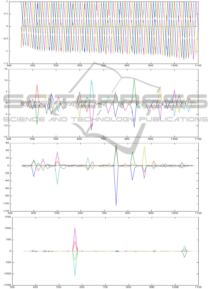
Figure 6: Obtention of the kernel K (in bottom row) of [p,r,g,b]

: R

→ R

. In each graph, respectively from above, 75,

74, 73 and 72 row vectors are plotted.

TetrachromaticMetamerism-ADiscrete,MathematicalCharacterization

BETA*AL2(ii+1,ii+1);

AL3(ii,ii+2)= AL2(ii,ii+2)/AL2(ii,ii)+ ...

BETA*AL2(ii+1,ii+2);

AL3(ii,ii+3)= BETA*AL2(ii+1,ii+3);

end

figure; plot(L,AL3)

\end{small}

AL4= zeros(76,72);

for ii=1:72

AL4(ii,ii)= 1;

BETA= -(P(ii) + P(ii+1)*AL3(ii,ii+1)/...

AL3(ii,ii) + P(ii+2)*AL3(ii,ii+2)/AL3(ii,ii)...

+ P(ii+3)*AL3(ii,ii+3)/AL3(ii,ii))/(P(ii+1)*...

AL3(ii+1,ii+1) + P(ii+2)*AL3(ii+1,ii+2) +...

P(ii+3)*AL3(ii+1,ii+3) + P(ii+4)*...

AL3(ii+1,ii+4));

AL4(ii,ii+1)= AL3(ii,ii+1)/AL3(ii,ii) + ...

BETA*AL3(ii+1,ii+1);

AL4(ii,ii+2)= AL3(ii,ii+2)/AL3(ii,ii) + ...

BETA*AL3(ii+1,ii+2);

AL4(ii,ii+3)= AL3(ii,ii+3)/AL3(ii,ii) + ...

BETA*AL3(ii+1,ii+3);

AL4(ii,ii+4)= BETA*AL3(ii+1,ii+4);

end

In the MATLAB code below, get 4x4 submatrix with

largest determinant, then get t (METAMER) for, e.g.

c = [

AL= transpose(AL);

iii=1

DETMAX= 0;

for ii = 1:73

for jj= ii+1:74

for kk = jj+1:75

for ll = kk+1:76

AL4x4=[AL(1, ii), AL(1,jj), AL(1,kk), AL(1, ll);...

AL(2, ii), AL(2,jj), AL(2,kk), AL(2, ll);...

AL(3, ii), AL(3,jj), AL(3,kk), AL(3, ll);...

AL(4, ii), AL(4,jj), AL(4,kk), AL(4, ll);];

DET= abs(det(AL4x4));

iii=iii+1;

if DET > DETMAX;

DETMAX= DET;

ii1=ii;

jj1=jj;

kk1=kk;

ll1=ll;

AL4= AL4x4;

end

iii= iii-1

AL4

det(AL4)

AL4INV=inv(AL4)

METAMER= AL4INV*[0.25;0.25;0.25;0.25]

4 TETRACHROMATIC HUE

METAMERISM

For us humans, two colours may have the same satu-

ration, the same luminance or the same hue. When

studying the colour vision of a tetrachromatic ani-

mal, it may be interesting to design an experiment

to ﬁnd out if the animal can distinguish hue while

disregarding luminance and saturation. In this sense,

we call two spectra hue-metameric if they give rise

to colour points on the same chromatic triangle (Re-

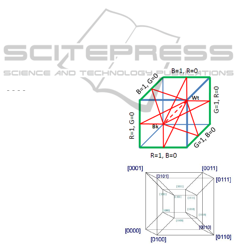
strepo, 2011); see Figure 7. In the colour hypercube

(Restrepo, 2012) you also have the achromatic seg-

ment and instead of a chromatic hexagon, you have

a chromatic icositetrahedron; the triangles having as

base the achromatic segment and as opposing a ver-

tex a point in the chromatic icositetrahedron are called

chromatic triangles and all colours in each such trian-

gle are said to have the same hue.

Figure 7: Chromatic triangles in RGB cube and hypercube.

VISAPP2014-InternationalConferenceonComputerVisionTheoryandApplications

5 CONCLUSIONS

Tetrachromacy and in particular tetrachromatic

metamerism is a subject well worth of attention. It

has applications both in computer vision and in the

modeling of biological vision systems. The subject

of tetrachromatic metamerism in computer vision has

applications for example in detection, in satellite im-

ages.

In our case, we have three types of cone pho-

topigment S(λ), M(λ) and S(λ) and it may be ar-

gued that from them, three other channels L + M + S,

(L+S)−M and (L+M)−S are derived. It is an inter-

esting fact of our colour vision that we have four per-

ceptual unique hues red, green, blue and yellow; per-

haps they are in a one-to-one correspondence with the

three channels S + L (”band-stop”), M (band-pass), S

(low-pass) and L + M (high-pass). The fact that the

L channel does not appear in an isolated form here,

might have to do with the fact that it was the last to

evolve.

It would be interesting to know how these facts ex-

trapolate in cases of the vision systems tetrachromatic

animals. One possibility is that they might perceive 6

unique hues, corresponding to the cases W + X (low-

pass), Y + Z (high-pass), X + Y (band-pass), W + Z

(stop-band) and, W +Y and X + Z (alternate band).

In a trichromatic context, (Cohen, 1964) has

shown how the reﬂectance spectra (samped at N=40

wavelengths) of a set of 150 Munsell chips, turned out

to be nearly three-dimensional; i.e. each spectrum is

nearly a linear combination of certain three spectra.

The analysis of large sets of natural reﬂectance spec-

tra surely gives interesting results.

In a tetrachromatic vision system, the use detector

with a bell response curve having a peak between

those of the S and M detectors, could prove to be

useful to differentiate between certain types of cyan

allowing the perception a certain type of cyan as a

unique and not as a combination of green and blue.

This would be certainly useful for marine vision

since short-wavelength light penetrates water more

than other wavelengths.

Typically, receptor curves are unimodal. In biol-

ogy, although not always in engineering as the exam-

ple in Section 3 shows, each receptor curve ”aperure-

samples” the visible spectrum, each sampling the en-

ergy in a, maybe overlapping, interval. In engineer-

ing, the use of detectors of comb spectra might be

useful as well.

ACKNOWLEDGEMENTS

We thank mathematician Ana Hern

andez for many in-

teresting discussions on the subject that helped to clar-

ify many ideas.

REFERENCES

Cohen, J. (1964). Dependency of the spectral reﬂectance

curves of the munsell color chips. Psychon Sci. , vol

1, pp.369-370.

Cohen, J. and Kappauf, E. (1982). Color stimuly, funda-

mental metamers and wyszecki’s metameric blacks.

The American Journal of Psychology, Vol. 95, No. 4,

pp. 537-564.

Jevbratt, L. (2013). Zoomorph - software simulating how

animals see. zoomorph.net.

Restrepo, A. (2011). Colour processing in runge space.

SPIE Electronic Imaging, San Francisco.

Restrepo, A. (2012). Tetrachromatic colour space. SPIE

Electronic Imaging, San Francisco.

Restrepo, A. (2013a). Colour processing in tetrachromatic

colour spaces. Visapp Rome.

Restrepo, A. (2013b). Hue processing in tetrachromatic

spaces. SPIE Electronic Imaging, San Francisco.

TetrachromaticMetamerism-ADiscrete,MathematicalCharacterization

REFERENCES

Cohen, J. (1964). Dependency of the spectral reflectance