
A Robust, Real-time Ground Change Detector for a “Smart” Walker
Viviana Weiss
1
, S
´
everine Cloix
1, 2
, Guido Bologna
1
, David Hasler
2
and Thierry Pun
1
1
Computer Science Department, University of Geneva, Route de Drize 7, Carouge, Switzerland
2
Vision Embedded Systems, CSEM SA, Jaquet Droz 1, Neuch
ˆ
atel, Switzerland
Keywords:
Ground Change Detection, Colour and Texture Segmentation, Local Edge Patterns (LEP), Artificial Neural
Network (ANN), Elderly Care, Gerontechnology.
Abstract:
Nowadays, there are many different types of mobility aids for elderly people. Nevertheless, these devices
may lead to accidents, depending on the terrain where they are being used. In this paper, we present a robust
ground change detector that will warn the user of potentially risky situations. Specifically, we propose a robust
classification algorithm to detect ground changes based on colour histograms and texture descriptors. In our
design, we compare the current frame and the average of the k previous frames using different colour systems
and Local Edge Patterns. To assess the performance of our algorithm, we evaluated different Artificial Neural
Networks architectures. The best results were obtained by representing in the input neurons measures related
to Histogram Intersections, Kolmogorov-Smirnov distance, Cumulative Integrals and Earth mover’s distance.
Under real environmental conditions our results indicated that our proposed detector can accurately distinguish
the grounds changes in real-time.
1 INTRODUCTION
The proportion of senior citizens have increased in
many countries; there are approximately 810 million
persons aged 60 years or over in the world in 2012 and
this number is projected to grow to more than 2 bil-
lions, by 2050 (United Nations, 2012). Loosing com-
plete or part of mobility, affects not only the ability
to walk but also the ability to perform personal tasks.
This is a major concern for life quality, which causes
dependence to others in daily life.
The proportion of old individuals living indepen-
dently currently represents 40% of the world’s pop-
ulation. This predominance is likely to increase in
the future, as people continue to get older. A severe
hindrance to independent living is decreased mobil-
ity, which might be due to health-related factors and
to sensory disability. Also, over a third of the popu-
lation aged 65 years and more falls at least once per
year; this ratio goes up to 50% for people over 80
years (Trombetti et al., 2009).
To help in their mobility, millions of people thus
use walkers (Fig.1). However, in several situa-
tions these devices fail to help and even contribute
to increase the likelihood of an accident. Typical
such problematic situations occur when the user mis-
judges the nature or the extent of particular obsta-
cles. This can happen both indoors and outdoors, and
both in familiar and unfamiliar environments. Vari-
ous prototypes of intelligent walkers were developed
(Dubowsky et al., 2000), (Frizera et al., 2008) and
(Rentschler et al., 2008); they are usually motorized,
aiming at route planning and obstacle detection, re-
lying on active sensing (laser, sonar, IR light) or on
passive sensing (RFID tags, visual signs). However,
such aids are usually expensive and only at the proto-
type level. For the end users, they represent complex
systems for which their acceptance is not necessar-
ily demonstrated. Their weight precludes easy trans-
portation and their autonomy is a weak point, often
limiting their use to indoor situations.
In this context, the goal of the EyeWalker project
is to develop a low-cost, ultralight computer vision
device for user with mobility problems. It would be
an inexpensive and independent accessory that could
simply be clipped on a standard walker. It should be
very easy to install by e.g. family members, and have
day-long autonomy. The goal of the EyeWalker de-
vice is to warn users of potentially risky situations or
help to locate a few particular objects, under widely
varying illumination conditions. The initial target
users would be elderly people that still live relatively
independently. After performing an analysis of user’s
requirements in three institutions for elderly people,
305
Weiss V., Cloix S., Bologna G., Hasler D. and Pun T..
A Robust, Real-time Ground Change Detector for a “Smart” Walker.
DOI: 10.5220/0004665703050312
In Proceedings of the 9th International Conference on Computer Vision Theory and Applications (VISAPP-2014), pages 305-312
ISBN: 978-989-758-004-8
Copyright
c
2014 SCITEPRESS (Science and Technology Publications, Lda.)

we have started working on ground change and obsta-
cles detection. The former is built on (Weiss et al.,
2013) and the latter is based on (Cloix et al., 2013).
In this paper, we focus on dangers at ground level,
such as holes, rugs, changes of terrain. The purpose
of this work is to develop a ground change detection
module that will warn the user before entering risky
situations.
Figure 1: Walker used in the study, equipped with a web-
cam and computer. It is a typical walker with four wheels,
handles with breaks and a seat
The main achievements of this paper are twofold.
The first one lies in the improvement of accuracy on
the detection of ground changes by integrating dif-
ferent techniques in an artificial neural network. The
second one lies on the feasibility of a robust detector
that works in real-time and outdoor situations. Our
key idea is based on the estimation of simultaneously
changes of brightness, color and textures under real
environmental conditions.
This paper is organized as follows: Section 2 dis-
cusses relevant work related to the state of the art in
autonomous navigation; Section 3 describes the pro-
posed approach to detect ground changes; Section 4
detail the hardware set-up proposed to evaluate the
performance of our method and discuss the results we
obtained. Finally, conclusions are given in Section 5.
2 RELATED WORK
Image processing for autonomous or assisted naviga-
tion in an unknown environment is a popular topic
that has been studied in robotics. Various works were
carried out using different hardware such as time of
flight sensors or radars or 3D stereoscopic imaging.
A few of the most common solutions in this setting
used edge detection or texture based classification to
separate different regions of ground.
The research described in (Lu and Manduchi,
2005) is focused on detecting physical edges on the
terrain, in order to find stairways and sidewalks. The
detection of such edges is made using both stereo-
scopic depth information and 2D image analysis.
The studies introduced by (Sung et al., 2010) use
a Daubechies wavelet transform on the images and
compute the features from the wavelet space for au-
tonomous mobility for military unmanned ground ve-
hicles in off-road environments. Other relevant work
carried out by (Liao et al., 2009), (Yao and Chen,
2003) and (Viet and Marshall, 2009) use distributions
of Local Edge Patterns (LBP). LBP is a commonly
used operator to extract textons and operates on a sub-
window in which it compares each pixel with a num-
ber of neighbours and returns a vector of binary val-
ues. The histogram of these vectors is then computed
for the current cell. The feature vector for the image is
the list of all these cell histograms. Studies on texture
classification indicate that LBP represents a relevant
feature (Ojala et al., 1996; Yang and Chen, 2013). Ex-
periments in (Pietikinen et al., 2004) also showed that
with LBP they obtained promising results on the clas-
sification of 3D surfaces under varying illumination
settings. The gray-scale invariability of LBP is also
used when considering outdoor scenarios.
Another way of classifying textures is by describ-
ing them through the use of textons, e.g. small el-
ements of texture information that can be learned
from the image. A common approach has been to
convolve a number of training images with a filter
bank and then cluster the filter responses to gener-
ate a dictionary. This texton dictionary is then used
to compute histograms of texton frequencies that rep-
resent the models of textures from the training im-
ages(Kang and Akihiro, 2013). Once this training has
been completed, a new image is classified using the
same method to generate the texton histogram from
the learned dictionary, and this histogram is com-
pared to the learned models. This method proved to
be effective in texture recognition (Li et al., 2012).
Some works, however, showed that the use of filter
banks might not be the optimal solution, arguing in
favour of features computed on smaller neighbour-
hoods (Varma and Zisserman, 2003).
3 METHODS
The main purpose of this research is to implement an
algorithm that detects a ground change in real time.
We propose a method based on the comparison be-
tween the current frame and the average of k previous
frames.
The procedure is divided in two different phases.
Firstly, we extract the image descriptor from the cur-
rent frame and the average of the k previous frames.
Secondly, we compare the descriptors with differ-
ent techniques and artificial neural networks architec-
tures. The block diagram to detect ground changes is
VISAPP2014-InternationalConferenceonComputerVisionTheoryandApplications
306
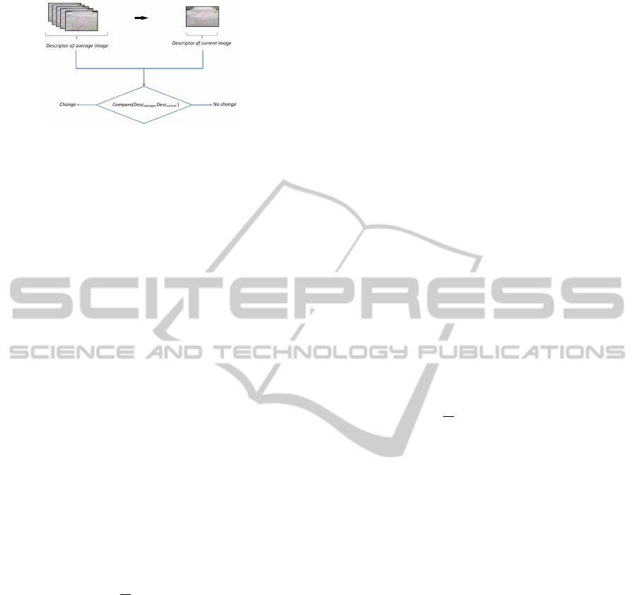
Figure 2: General block diagram to detect ground changes.
illustrated in Fig.2.
The extraction of features distributions is de-
scribed in Section 3.1 and latter is explained differ-
ent methods to measure the similarity between the de-
scriptors in Section 3.2.
3.1 Image Descriptor
Image descriptors used in this work are based on usual
metrics like color and brightness.
Two kind of features distributions are applied as
texture descriptor: Colour feature and Texture feature.
Both are extracted from each image in order to mea-
sure their similarity.
3.1.1 Colour Feature
In this study, different colour spaces like RGB, HSV,
CieLAB, YCbCR, Ntsc and grayscale were system-
atically assessed in the experiments. The evaluation
results with HSV demonstrated to be more satisfac-
tory, as shown in the results on Section 4.
From the image, we obtain the normalized colour
histogram h
c
for each colour channel using the fol-
lowing equation:
h
H,S,V
c
i
=
n
i
N
, i = 0, . . . , 255 (1)
where n
i
is the number of pixels with colour label i
and N is the total number of pixels in the image for
each channel.
3.1.2 Texture Feature
The Local Binary Patterns (LBP) value is defined as
(Yao and Chen, 2003),
LBP(n, m) =
∑
i, j∈I
k(i, j)×u( f (n+i, m + j)− f (n, m)),
(2)
where k is the LBP mask:
k(i, j) =
1 2 4
8 0 16
32 64 128
(3)
The idea of LBP was adapted to define the Local
Edge Pattern (LEP). LEP describes the spatial struc-
ture of the local texture according to the organization
of edge pixels. To compute the LEP histogram, an
edge image must be obtained first. The edge image
is obtained by applying the Sobel edge detector to in-
tensity gray level. The binary values are then multi-
plied by the corresponding binomial weights in a LEP
mask, and the resulting values are summed to obtain
the LEP value.
The LEP value is defined as (Kumar and Gupta,
2012),
LEP(n, m) =
∑
i, j∈I
K
e
(i, j) × I
e
(n, m) (4)
where I
e
(n, m) denote the binary image, K
e
is the LEP
mask and LEP(n, m) is the LEP value for the pixel
(n, m). The LEP mask is given by:
K
e
=
1 2 4
128 256 8
64 32 16
(5)
Finally, the LEP normalized histogram h
e
can be
computed from
h
e
i
=
n
i
N
, i = 0, . . . , 511 (6)
where n
i
is the number of pixels with LEP value i and
N is the total number of pixels in the image.
3.2 Ground Change Detection
The colour’s distribution and LEP are used to obtain
a distance measure between two images characteris-
ing the inhomogeneity of a surface. Specifically, this
is calculated between the current image and the av-
erage of the k previous images. There are different
ways of measuring the similarity between frames (Pe-
natti et al., 2012). In order to distinguish the ground
change, we implemented the following four methods
using some of the most common distance functions.
3.2.1 Histogram Intersection (HI)
Histogram Intersection is used to compare image de-
scriptors. It calculates the sum of overlapping areas
between two histograms (Viet and Marshall, 2009).
The homogeneity measure H
di f f
of two images is de-
fined by:
H
di f f
=
∑
i
min(hist
current
i
, hist
average
i
) (7)
in which hist
current
and hist
average
are current and av-
erage histograms, hist
current
i
is the value of bin i in
ARobust,Real-timeGroundChangeDetectorfora"Smart"Walker
307
hist
current
. The closer H
di f f
is to 1, the more alike the
current histogram and the average histogram are.
3.2.2 Kolmogorov-Smirnov Distance (KS)
The Kolmogorov-Smirnov distance measures the dis-
similarity between two distributions. The smaller this
dissimilarity value the more identical the two distri-
butions are (Puzicha et al., 1999). In order to cal-
culate the dissimilarity value the absolute difference
between the histograms is given by:
D(H
a
, H
c
) = max |F(H
a
) − F(H
c
)| (8)
where H
a
and H
c
are average and current histograms
respectively and D(H
a
, H
c
) is the dissimilarity be-
tween these histograms. F(H
a
) and F(H
c
) are the
distributions of normalized histograms for H-, S-, V-
channel and LEP.
3.2.3 Cumulative Integral (CI)
The Cumulative Integral compares histograms by
building the cumulative distribution function of each
histogram, and comparing these two functions.
The cumulative distribution function f
i
for n bins
of the histogram H
i
is defined as:
f
i
(n) =
1
n
n
∑
i=0
H
i
(n) (9)
and the dissimilarity measure is given by:
D(H
a
, H
c
) = |σ( f (H
a
) − σ( f (H
c
)| (10)
where σ( f (H
a
) and σ( f (H
c
) are the standard devia-
tion of average and current histograms distributions
respectively. The smaller the dissimilarity D(H
a
, H
c
)
the more identical the two distributions are.
3.2.4 Neural Networks (NN) based on Features
Fusion
We consider a three multilayer perceptron with n neu-
rons in the input layer, l neurons in the hidden layer
and m neurons in the output layer. In a first series of
experiments we take into account the values of each
bin in the histograms (H,S,V channels and LEP) as
input layer. As we have three colour channels, each
channel having 256 bins and a texture channel rep-
resented by 512 bins, the input vector of our neural
network contains 2560 neurons (Fig. 3). The size of
the hidden layer is determined empirically (see Sect.
4), whereas the output layer has two neurons, one rep-
resenting the detection of the ground change and the
other indicating unchanged ground.
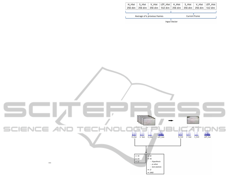
In a second series of experiments we reduce the
size of the input layer by just taking into account the
Figure 3: Description of the input vector for the first series
of experiments.
histogram similarity measures described in the previ-
ous sub-sections (see Sect. 3.2.1,3.2.2,3.2.3). We im-
plemented two methods; in the first one, we used the
similarity measure between each histogram (H,S,V
and LEP) to calculate HI, the binary value for simi-
larity of the KS and CI. The input vector of this ANN
has 12 neurons. For the second method we have again
global measures related to histograms and we include
three values for the test of Kolmogorov-Smirnov (bi-
nary value for similarity, p-value and test statistic) and
the Earth mover’s distance (EMD) shown in Fig. 4.
The input vector has 24 neurons for this method.
Figure 4: Block diagram for obtaining values used as input
vector in our NN with 12 and 24 neurons.
4 EXPERIMENTS & DISCUSSION
A set of outdoor video sequences were collected from
a campus path at Geneva University using the walker
shown in Fig.1; Fig.5 presents some typical situa-
tions to be detected. This data set was recorded with
a walker equipped with a colour webcam (Logitech
HD Webcam C510, 8 Mpixels) located 60 cm from
the ground. The covered visual field region is about
130 cm long, as shown in Fig.6. We use a total of
six videos recorded at different times, each video con-
taining between 188 and 313 frames and two to four
ground change transitions. Note that videos were
recorded at an approximative speed of 0.6 m/s (2.3
km/h) with a frame rate of 25 f ps.
To assess the performance of our approach, an ex-
tensive and systematic evaluation in terms of accuracy
and processing time of colour space, similarity mea-
sures and artificial neural networks architectures were
conducted on a data set labelled manually.
VISAPP2014-InternationalConferenceonComputerVisionTheoryandApplications
308
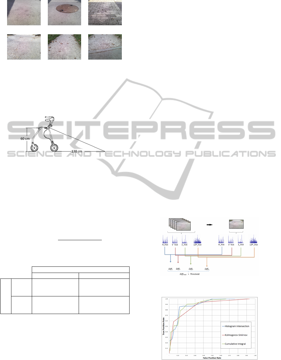
(a) (b) (c)
(d) (e) (f)
Figure 5: Ground change images extracted from the test
video sequences; six different situations are presented: (a)
and (d) represent a typical example of the path but with dif-
ferent texture, (b) represents a path with an obstacle, (c)
represents a non uniform surface, (e) represents a delimited
path and (f) represents a path with a ground change.
Figure 6: Actual hardware set-up allowing detecting ground
changes at less than 1.30 meters.
The two classes, ground change and no change,
are defined as follows: a frame is labelled positive as
soon as a ground change enters the visual field and
it remains positive until the user is completely on the
new terrain; the frame is labelled negative otherwise.
To compare the methods, we use the confusion matrix
shown in Table 1, where accuracy is define as:
Accuracy =
t p +tn
t p +tn + f p + f n
(11)
Table 1: Terminology use for the evaluation.
Condition
Ground change No change
System result
Ground
change
True positive “tp”
(Correct alarm)
False Positive “fp”
(Unexpected alarm)
No
change
False negative “fn”
(Missing alarm)
True negative “tn”
(Correct absence of
alarm)
In our system, the most critical value is the miss-
ing alarm because it can generate an accident. We
however must minimize the false positive rate to en-
sure user acceptance.
4.1 Evaluation of Features
We tested 6 different colours spaces: RGB, HSV,
CieLab, Ntsc, YCbCr and Grayscale. To determine
the number of k previous frames used in our algo-
rithm, we tried different values between 1 to 25. The
results shown on Table 2 were obtained using his-
togram intersection to measure the dissimilarity be-
tween different histograms.
The purpose of this first experiment is to compare
different colour spaces and to determine the number
of k previous frames. The HSV colour system with
k = 5 presents the best performance with an accuracy
of 85.4%.
4.2 Evaluation of Different Similarity
Measure Methods
Colour information is sometimes not sufficient to de-
tect ground changes. The majority of detection errors
appear when the images are under variable illumina-
tion conditions, or when a shadow enters in the visual
field. To reduce this type of errors, we implemented a
robust detector which takes into account texture fea-
tures described in Section 3.1. From this observa-
tion, the three colour channels (H,S and V) and LEP
are used to derive a similarity measure between the
frames. Fig.7 shows the proposed method that incor-
porates colour and texture features in a unified way.
To measure the dissimilarity between each histogram,
we used the techniques described in Section 3.2.
The results shown on Fig.8 and Table 3 were ob-
tained by calculating the average of the homogene-
ity measure between the histograms. To compute the
Figure 7: Block diagram to compare each histogram in or-
der to measure the dissimilarity between the frames.
Figure 8: Performance of the usual methods. Receiver oper-
ating characteristic (ROC) curves of Histogram Intersection
(blue), the Kolmogorov-Smirnov distance (red) and the Cu-
mulative Integral (green) with k = 5.
ARobust,Real-timeGroundChangeDetectorfora"Smart"Walker
309
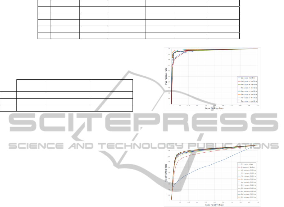
Table 2: Comparison of accuracy using different colour spaces and k average images.
k RGB (%) HSV (%) CIELAB (%) NTSC(%) YCbCr(%) GRAY(%)
1 75.42 77.16 70.86 75.00 75.50 75.00
3 77.97 79.94 70.63 76.03 76.40 76.03
5 81.98 85.36 74.05 78.67 76.08 73.67
10 73.18 75.28 68.48 69.80 68.90 69.80
25 72.38 71.28 70.83 70.17 76.28 70.17
Table 3: Comparison of dissimilarity measures between the
images. In order to detect ground changes, we applied a
threshold of 0.05 for Histogram Intersection (HI), 0.6 for
Kolgomorov-Smirnov (KS) and 0.006 for Cumulative Inte-
gral (CI).
Accuracy
(%)
False alarm
detection (%)
Missing alarm
rate (%)
HI
87.45 11.89 14.29
KS
84.87 4.90 41.70
CI
84.66 12.93 21.62
resulting performance of different methods, we used
the accuracy, the false alarm detection (False positive
rate) and the missing alarm rate (False negative rate).
As a result, we found that the three methods present a
similar accuracy, but the most important difference is
in the missing alarm rate: Histogram Intersection per-
forms approx. 7% better than the Cumulative Integral
and approx. 27% than the Kolmogorv-Smirnov.
4.3 Evaluation of Different NN
Architectures
To evaluate the different NN architectures we per-
formed a ten-fold cross-validation by creating 10 dif-
ferent training/validation pairs by sliding the training
data window by 10% each time. Then, for each of
the training/validation pair, we performed 10 classi-
ficatory runs. We trained each run using the corre-
sponding training set. Afterwards, we evaluated the
classification using the rest of the dataset. Therefore,
a total of 100 runs is performed per experiment.
To determine the number of hidden units used in
our networks, we tried different number of neurons in
the hidden layer and performed a training/validation
procedure using the whole dataset. From these re-
sults, we chose for each architecture, the best number
of hidden units (i.e., the one that minimizes the clas-
sification error).
Fig. 9 shows the performance of our system with
a NN that uses all bins of the H, S, V and LEP
histograms (2560 neurons) in the input layer (see
Sect.3.2.4); we modified the number of neurons in the
hidden layer between one to eight neurons. We found
that the best set of results was given by six neurons.
In order to reduce the neural network complexity
(number of input neurons), we implemented NN ar-
Figure 9: NN performance with an input vector of 2560
neurons. ROC curves with different number of neurons (be-
tween 1 to 8) for the hidden layer. We compare the current
frame with the average of the k = 5 previous frames.
Figure 10: NN performance with an input vector of 12 neu-
rons in the input layer. ROC curves with different number
of neurons (between 1 to 55) for the hidden layer. We com-
pare the current frame with the average of the k = 5 previous
frames.
chitectures that used three histogram similarity mea-
sures for each histogram (H,S,V channel and LEP)
instead of all bins of the histograms. Sect. 3.2.4 ex-
plained how we reduced the input layer. The results
shown at Fig.10 were obtained by using 12 neurons in
the input layer and varying the value of neurons in the
hidden layer between 1 to 55 neurons. We found that
the best results were achieved with 45 neurons in the
hidden layer.
The results demonstrate it is not an improvement
(accuracy from 97.29% to 90.94%, false alarm de-
tection from 1.59% to 5.54% and missing alarm rate
from 5.96% to 8.49%) when we reduce the input vec-
tor from 2560 to 12 neurons. To assess the perfor-
mance obtained with a NN that used 12 neurons in
the input layer, we implemented a neural network that
uses six histogram similarity measures for each his-
togram (H,S,V channel and LEP), the input vector
VISAPP2014-InternationalConferenceonComputerVisionTheoryandApplications
310
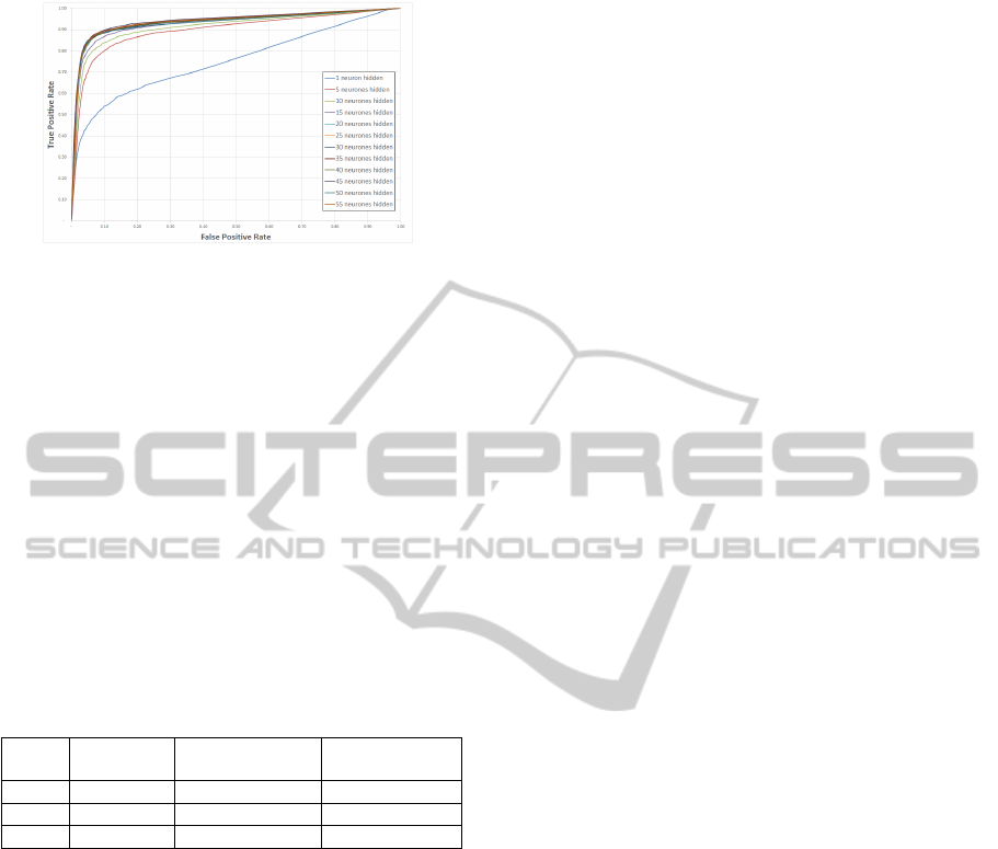
Figure 11: NN performance with an input vector of 24 neu-
rons in the input layer. ROC curves with different number
of neurons (between 1 to 55) for the hidden layer. We com-
pare the current frame with the average of the k = 5 previous
frames.
has 24 neurons. The results shown at Fig.11 were
obtained by using 24 neurons in the input layer and
varying the value of neurons in the hidden layer be-
tween 1 to 55 neurons. The best performance was
given by using 30 neurons in the hidden layer.
The results of the different architectures with the
best values of neuron numbers in the hidden layer are
reported in Table 4.
Table 4: Comparison of methods using different NN archi-
tectures, where n is the number of neurons in the input layer.
The numbers of neurons in the hidden layer are 6 for 2560
neurons in the input layer, 30 for 24 neurons in the input
and 45 for 12 neurons in the input layer.
n
Accuracy
(%)
False alarm
detection (%)
Missing alarm
rate (%)
2560 97.29 1.59 5.96
24 92.41 4.09 1.47
12 90.94 5.54 8.49
These results show that the best missing alarm rate
is obtained when we implemented a fusion of dissim-
ilarity measures with 24 neurons in the input layer.
Besides, the implementation a fusion of measures
in a NN with 24 neurons in the input enables a signif-
icant improvement in comparison with a usual simi-
larity measure like Histogram intersection (accuracy
from 87.45% to 92.41%, false alarm detection from
11.89% to 4.09% and missing alarm rate from 14.29%
to 1.47%).
4.4 Evaluation of Processing Time
An evaluation criteria is the processing time between
the input image and the instant of detection. In
these experiments, the average of processing time for
HI,KS and CI is approx. 0.1 s, whereas for the NN is
approx. 0.2 s computed in Matlab
R
R2013a by using
a Dell computer with an Intel(R) Core(TM) i7-2600
CPU 3.40GHz.
Finally, it must be remarked that the latency be-
tween the frame where the ground change appears
on the top of the visual field and the frame where it
is actually detected, is important in our system be-
cause it shows us the viability to implement our detec-
tor in the real world. The average latencies obtained
where the following: using Histogram Intersection,
10 frames (approximately equivalent to 25 cm); the
Kolmogorov-Smirnov, 27 frames (70 cm); the Cumu-
lative Integral, 14 frames (40 cm); and last the Neural
Networks, 1 frame (6 cm). Based on these results,
we conclude that NN achieve the best performance in
terms of latency.
5 CONCLUSIONS
Early detection of sudden changes in terrain is ex-
tremely important for walkers users, it can present se-
rious challenges to user balance. In this paper, we
have presented a robust and real-time ground change
detector to warn walker’s users before entering dan-
gerous terrains. This detector was built using the com-
parison between current and past frames. The method
proposed uses a fusion of dissimilarity measures with
a Neural Network.
The main results of our research show that a
significant improved performance can be obtained
when combining different measures. The experiments
demonstrate that the fusion of measures gives im-
provement in the accuracy of about 10% compared
to usual dissimilarity measures like Histogram Inter-
sections, Kolmogorov-Smirnov distance or Cumula-
tive Integral. Our studies show that artificial neural
networks achieved the best performances in terms of
false alarms, missing alarms and the latency of the
system.
Further work will be done in order to predict pos-
sible dangerous situations by studying the user’s be-
haviour. We plan to assess the user’s behaviour using
a motion vector and ground information.
Finally, the experiments show promising results
which reflect that our ground change detector can be
possible used in an embedded device with high likeli-
hood of good performance in real situations.
ACKNOWLEDGEMENTS
This work has been developed as part of the Eye-
Walker project that is financially supported by the
Swiss Hasler Foundation Smartworld Program, grant
Nr. 11083.
We thank our end-users partner the FSASD,
ARobust,Real-timeGroundChangeDetectorfora"Smart"Walker
311

Fondation des Services d’Aide et de Soins Domi-
cile, Geneva, Switzerland; EMS-Charmilles, Geneva,
Switzerland; and Foundation “Tulita”, Bogot
´
a,
Colombia.
REFERENCES
Cloix, S., Weiss, V., Bologna, G., Pun, T., and Hasler,
D. (2013). Object detection and classification us-
ing sparse 3d information for a smart walker. Poster
Session in Swiss Vision Day 2013 SVD’13, Zurich,
Switzerland.
Dubowsky, S., Genot, F., Godding, S., Kozono, H., Skwer-
sky, A., Yu, H., and Yu, L. S. (2000). Pamm - a robotic
aid to the elderly for mobility assistance and monitor-
ing: a ”helping-hand”; for the elderly. In Robotics and
Automation, 2000. Proceedings. ICRA ’00. IEEE In-
ternational Conference on, volume 1, pages 570–576.
Frizera, A., Ceres, R., Pons, J. L., Abellanas, A., and Raya,
R. (2008). The smart walkers as geriatric assistive de-
vice. the simbiosis purpose. In Gerontechnology, vol-
ume 7, page 108.
Kang, Y. and Akihiro, S. (2013). Texton clustering for local
classification using scene-context scale. In Frontiers
of Computer Vision, (FCV), 2013 19th Korea-Japan
Joint Workshop on, pages 26–30.
Kumar, P. and Gupta, V. (2012). Learning based obstacle
detection for textural path. In International Journal
of Emerging Technology and Advanced Engineering,
volume 2, pages 436–439.
Li, X.-Z., Williams, S., Lee, G., and Deng, M. (2012).
Computer-aided mammography classification of ma-
lignant mass regions and normal regions based on
novel texton features. In Control Automation Robotics
Vision (ICARCV), 2012 12th International Conference
on, pages 1431–1436.
Liao, S., Law, M., and Chung, A. (2009). Dominant lo-
cal binary patterns for texture classification. In Image
Processing, IEEE Transactions on, volume 18, pages
1107–1118.
Lu, X. and Manduchi, R. (2005). Detection and localization
of curbs and stairways using stereo vision. In Robotics
and Automation, 2005. ICRA 2005. Proceedings of the
2005 IEEE International Conference on, pages 4648–
4654.
Ojala, T., Pietikainen, M., and Harwood, D. (1996). A com-
parative study of texture measures with classification
based on featured distributions. In Pattern Recogni-
tion, volume 29, pages 51 – 59.
Penatti, O. A., Valle, E., and da S. Torres, R. (2012). Com-
parative study of global color and texture descriptors
for web image retrieval. In Journal of Visual Commu-
nication and Image Representation, volume 23, pages
359 – 380.
Pietikinen, M., Nurmela, T., Menp, T., and Turtinen, M.
(2004). View-based recognition of real-world tex-
tures. In Pattern Recognition, volume 37, pages 313 –
323.
Puzicha, J., Buhmann, J., Rubner, Y., and Tomasi, C.
(1999). Empirical evaluation of dissimilarity mea-
sures for color and texture. In Computer Vision, 1999.
The Proceedings of the Seventh IEEE International
Conference on, volume 2, pages 1165–1172.
Rentschler, A. J., Simpson, R., Cooper, R. A., and
Boninger, M. L. (2008). Clinical evaluation of guido
robotic walker. In Journal of rehabilitation research
and development, volume 45, pages 1281–1293.
Sung, G.-Y., Kwak, D.-M., and Lyou, J. (2010). Neural
network based terrain classification using wavelet fea-
tures. In Journal of Intelligent & Robotic Systems,
volume 59, pages 269–281. Springer.
Trombetti, A. et al. (2009). Pr
´
evention de la chute: un enjeu
de taille dans la strat
´
egie visant
`
a pr
´
evenir les fractures
chez le sujet
ˆ
ag
´
e. In Ost
´
eoporose, volume 207, pages
1318–1324. M
´
edecine et Hygi
`
ene.
United Nations (2012). Population ageing and devel-
opment 2012. Available at http://www.un.org/en/
development/desa/population/publications/pdf/ageing/
2012PopAgeingandDev WallChart.pdf.
Varma, M. and Zisserman, A. (2003). Texture classifi-
cation: Are filter banks necessary? In Computer
vision and pattern recognition, 2003. Proceedings.
2003 IEEE computer society conference on, volume 2,
pages 691–698. IEEE.
Viet, C. N. and Marshall, I. (2009). An efficient obstacle
detection algorithm using colour and texture. In Pro-
ceedings of World Academy of Science Engineering
and Technology, volume 60, pages 123–128.
Weiss, V., Cloix, S., Bologna, G., Pun, T., and Hasler, D.
(2013). A ground change detection algorithm using
colour and texture for a smart walker. Poster Session
in Swiss Vision Day 2013 SVD’13, Zurich, Switzer-
land.
Yang, B. and Chen, S. (2013). A comparative study on lo-
cal binary pattern (lbp) based face recognition: {LBP}
histogram versus {LBP} image. In Neurocomputing,
volume 120, pages 365 – 379.
Yao, C.-H. and Chen, S.-Y. (2003). Retrieval of translated,
rotated and scaled color textures. In Pattern Recogni-
tion, volume 36, pages 913 – 929.
VISAPP2014-InternationalConferenceonComputerVisionTheoryandApplications
312
