Likelihood Functions for Errors-in-variables Models

Bias-free Local Estimation with Minimum Variance

Kai Krajsek, Christian Heinemann and Hanno Scharr

IBG-2: Plant Sciences, Forschungszentrum J

ulich, 52425, J

ulich, Germany

Keywords:

Parameter Estimation, Maximum Likelihood Estimation, Error-in-Variables Models, CRLB, Optical Flow.

Abstract:

Parameter estimation in the presence of noisy measurements characterizes a wide range of computer vision

problems. Thus, many of them can be formulated as errors-in-variables (EIV) problems. In this paper we

provide a closed form likelihood function to EIV problems with arbitrary covariance structure. Previous

approaches either do not offer a closed form, are restricted in the structure of the covariance matrix, or involve

nuisance parameters. By using such a likelihood function, we provide a theoretical justiﬁcation for well

established estimators of EIV models. Furthermore we provide two maximum likelihood estimators for EIV

parameters, a straight forward extension of a well known estimator and a novel, local estimator, as well as

conﬁdence bounds by means of the Cramer Rao Lower Bound. We show their performance by numerical

experiments on optical ﬂow estimation, as it is well explored and understood in literature. The straight forward

extension turned out to have oscillating behavior, while the novel, local one performs favorably with respect

to other methods. For small motions, it even performs better than an excellent global optical ﬂow algorithm

on the majority of pixel locations.

1 INTRODUCTION

Major computer vision problems, e.g. optical ﬂow

estimation (Lucas and Kanade, 1981), camera cali-

bration (Clarke and Fryer, 1998), 3D rigid motion

estimation (Matei and Meer, 2006), or ellipse ﬁt-

ting (Kanatani, 2008) can be described by errors-in-

variables (EIV) models. EIV models are generaliza-

tions of regression models, accounting for measure-

ment errors in the independent, measured variables. It

is well known, that a wide range of least squares esti-

mation schemes are of this type (see (Markovsky and

Huffel, 2007) for a recent overview), e.g. total least

squares estimation (TLS), weighted TLS, or general-

ized TLS.

Characteristic of such models is the coupling of

the variables of interest with the measurement noise.

E.g. spatio-temporal image derivatives needed to esti-

mate optical ﬂow in a differential estimation scheme,

not only suffer from image noise, but also this noise is

correlated by the convolution kernels applied to calcu-

late the derivatives. As a consequence more sophisti-

cated regression techniques than simple least squares

approaches have to be applied in order to obtain re-

liable estimation results. Using such an estimation

scheme well adapted to the requirements of a speciﬁc

application can make a signiﬁcant difference in terms

of accuracy and reliability of the results (see Fig. 1

for an optical ﬂow example).

Most prominent among these regression tech-

niques are maximum likelihood (ML) estimators. ML

estimation is a well established estimation technique

known to be asymptotic efﬁcient, meaning that it is

asymptotically unbiased and has asymptotically the

lowest possible variance for an unbiased estimator

(cmp. Sec. 2).

For identical independent distributed (iid) Gaus-

sian noise in all measurements the ML estimator is

known to be equal to TLS (Abatzoglou et al., 1991;

Huffel and Lemmerling, 2002). Unfortunately, the iid

requirement is not always fulﬁlled in practice. Thus

applying TLS also leads to biased results. Violation

of the iid assumption can be either due to correlations

between different measurements, as in the OF exam-

ple above, or due to varying noise levels, as e.g. in low

light scenarios, where the noise strongly depends on

image intensities.

Our Contribution. We provide a likelihood

function for EIV models, generalizing and simpli-

fying previous approaches (Matei and Meer, 2006;

Kanatani, 2008; Chojnacki et al., 2001; Leedan and

Meer, 2000). The connection to our approach is dis-

270

Krajsek K., Heinemann C. and Scharr H..

Likelihood Functions for Errors-in-variables Models - Bias-free Local Estimation with Minimum Variance.

DOI: 10.5220/0004667402700279

In Proceedings of the 9th International Conference on Computer Vision Theory and Applications (VISAPP-2014), pages 270-279

ISBN: 978-989-758-009-3

 2014 SCITEPRESS (Science and Technology Publications, Lda.)

20 40 60 80 100 120 140

0.2

0.4

0.6

0.8

20 40 60 80 100 120 140

0.2

0.4

0.6

0.8

20 40 60 80 100 120 140

0.2

0.4

0.6

0.8

20 40 60 80 100 120 140

0.2

0.4

0.6

0.8

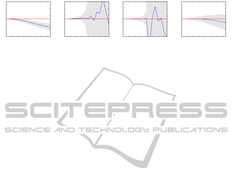
Figure 1: Results for synthetic sinusoidal pattern moving with velocity u = 0.5. Mean (blue curve) and variance (gray area)

vs. noise level of the image sequence. Left to right: LS (e.g. (Lucas and Kanade, 1981)), TLS (e.g. (Nestares et al., 2000;

Nestares and Fleet, 2003)), equilibration (M

uhlich and Mester, 2004), our approach. We observe less bias for our method

wrt. LS. Lower variance of LS is due to its bias. We further see much less variance compared to TLS and equilibration. For

details see Sec.4.

cussed in detail. Furthermore we derive two schemes

enabling to statistically optimal estimate parameters

and give a method for estimating conﬁdence bounds

in terms of the Cramer-Rao lower bound (CRLB).

Bias and variance behavior are compared, as well as

the stability of our algorithms to TLS (e.g. (Nestares

et al., 2000; Nestares and Fleet, 2003)) and equilibra-

tion (M

uhlich and Mester, 2004) using random EIV

systems of equations and a toy optical ﬂow problem.

In addition we show that, in well-structured image

regions, our estimates compare favorable to one of

the best-performing variational, so-called global al-

gorithms (Sun et al., 2010) on the Middlebury test set

(Baker et al., 2007). This demonstrates that using a

local estimator can be beneﬁcial, when interested in

highest accuracy in the presence of ’good data’. The

derived CRLB allows to detect these good estimates.

Related Work. There is a rich literature on dif-

ferent LS methods, suitable algorithms and their error

bounds. Markovsky and Van Huffel (Markovsky and

Huffel, 2007) give an overview of variants of TLS

estimation, e.g. Weighted TLS, Generalized TLS,

or Structured TLS. Lemmerling et al. (Lemmerling

et al., 1996) show the equivalence of Constrained TLS

and Structured TLS. Yeredor (Yeredor, 2000) formu-

lates a more general criterion called Extended LS

(XLS), where LS, TLS, Constrained TLS and Struc-

tured TLS are special cases of XLS. Robust variants

like robust MSE (Mean Square Error) (Eldar et al.,

2005), or structured robust LS, minimize the worst

case residual over a set of perturbations structured

with constant sets of data matrices and vectors.

Numerous approaches have been proposed to

compensate for the bias in the TLS estimator when

noise is correlated and some of them claim to provide

an ML estimator (Nagel, 1995; M

uhlich and Mester,

2004; Andres et al., 2008) but non of these estimators

delivers an analytical model for the likelihood func-

tion.

Current approaches providing closed form likeli-

hood functions suffer either from nuisance parame-

ters increasing the dimensionality of the likelihood

function with the number of measurements, or im-

pose rather strong restrictions on the error structure

of the measurements, e.g. errors of different measure-

ments are mutually statistically independent. Simon-

celli (e.g. (Simoncelli, 1993)) derived a (conditioned)

likelihood function without noise coupling to the pa-

rameters. Nestares (Nestares et al., 2000; Nestares

and Fleet, 2003) derived a closed form likelihood

function assuming the noise of different measurement

to be statistically independent.

2 MAXIMUM LIKELIHOOD

ESTIMATION

Let us repeat some basic notions of estimation the-

ory needed in the remainder of the paper. Denote

with {g

}, i = {1, ...,m}, m observations, with g =

;...;g

) the vector containing all observations

and with u a real valued parameter vector to be es-

timated. An estimator denotes a rule for assigning a

parameter vector ˆu for a given set of observations g.

Furthermore, let us denote with p(g|u) the sampling

distribution of the observations. Considering the sam-

pling distribution as a function of the parameter vector

u for a given set of observations yields the likelihood

function L : u 7→ p(g|u).

Important characterizations of estimators are

given by the terms consistency, (un)biased, variance,

efﬁciency and the Cramer Rao lower bound (CRLB).

Loosely speaking, an estimator is called consistent if

its estimates converge in a probabilistic sense to the

true parameter for increasing number of observations.

An estimator is called unbiased if the mean of its es-

timates equals the true value of the parameters u

, re-

peating the experiment inﬁnitely often. The quality of

an (unbiased) estimator is measured by means of its

variance, i.e. a lower variation around the true value

is considered as more reliable. Naturally one seeks for

the estimator with lowest possible variance, irrespec-

tive of the considered data, known as the minimum

LikelihoodFunctionsforErrors-in-variablesModels-Bias-freeLocalEstimationwithMinimumVariance

271

variance unbiased estimator (MVUE). The CRLB ex-

presses a lower bound on the variance σ

of an un-

biased estimator, given by the inverse of the Fisher

Information I(u

)

≥ I

−1

) with I(u

) = −E[∂

(log(p(g|u)))] (1)

The quotient between the CRLB and the variance

achieved by an estimator is called efﬁciency. Thus if

an estimator is unbiased and achieves the CRLB, then

it is an MVUE. On the other hand if an estimator has

a lower variance than the CRLB it must be biased.

There is no general rule for deriving an MVUE

or even an efﬁcient estimator. However, if measure-

ments are independent distributed the maximum like-

lihood estimator

ˆu = arg

max

∏

p(g

|u) (2)

is known to be asymptotically efﬁcient, i.e. for m → ∞

it is unbiased and it attains the CRLB. Unfortunately,

for the general case of EIV models, like e.g. in optical

ﬂow estimation, measurements cannot be assumed to

be independent such that asymptotic results cannot be

applied. In this case, the maximum likelihood func-

tion can still be applied within a Bayesian context,

e.g. maximum a posteriori (MAP) or minimum mean

squared estimation. Considering a ﬂat prior distribu-

tion, the likelihood function is proportional to the pos-

terior pdf. If the posterior is not too skewed, the MAP

estimate is a reasonable point estimator of the param-

eters and its variance an estimator of the conﬁdence

of that point estimate.

By deriving the likelihood function for the EIV

models we design an (asymptotically) unbiased, efﬁ-

cient estimator with a natural conﬁdence measure by

means of the CRLB.

3 ERRORS-IN-VARIABLES

PROBLEMS

Notation. Two different notations for EIV-

problems are common in literature, the one using

homogeneous coordinates for the parameter vector of

interest, the other using Cartesian coordinates. We

introduce both notations as they suggest different

estimation schemes, i.e. our Type I and Type II

schemes.

Using homogeneous coordinates for the parameter

vector u, the observation equations can be given by

u = 0 (3)

with i = 1, ...,m factorizing in i vectors of noise-free

true values g

. As the parameters in u are freely scal-

able they usually are restricted to the unit sphere S

n−1

i.e. |u| = 1. Assuming additive noise on the obser-

vations, i.e. g

= g

+ η

, we observe that the noise

couples to the parameter vector

u − η

u = 0 . (4)

As u is deﬁned on the unit sphere, at least one compo-

nent is nonzero. If u is known, we can assume u

6= 0

and divide (4) by u

. This allows (3) and (4) to be re-

formulated using a second frequently used notation,

where parameter vector w is given in Cartesian coor-

dinates

w + b

= 0 and a

w + b

= ρ

(5)

with a

, a

, w ∈ R

n−1

, and ρ

, b

∈ R and i =

1,..., m, and further error components ρ

= η

u/u

observations

= ((g

)

,..., (g

)

n−1

)

, b

= (g

)

, (6)

true values

= ((g

)

,..., (g

)

n−1

)

, b

= (g

)

, (7)

and scaled parameter vector

w = (u

,..., u

n−1

)

. (8)

These condition equations can be compactly writ-

ten with the matrix vector notation as

Aw + b = ρ and A

w + b

= 0 (9)

where we introduced the vectors

b = (b

,..., b

)

, b

= (b

,..., b

)

ρ = (ρ

,..., ρ

)

(10)

and the m × n-matrices A and A

whose i-th column

contains the vector a

and a

, respectively.

Let us further introduce the vectors a = Vec(A)

and a

= Vec(A

). Note that some authors, e.g.

(Nestares et al., 2000; Nestares and Fleet, 2003), also

start their analysis with this form (5) of the observa-

tion equations.

3.1 The EIV Likelihood Function

A known way (Gleser, 1981) to derive a likelihood

function L : (w, a

) 7→ p(a, b|w,a

) for the EIV prob-

lem (5) is to make the variable transformation η

→

− a

− b

) in the noise model p({η

}) and use

= −a

w from the ﬁrst Equation in (5) to elim-

inate b

. The disadvantage of this likelihood func-

tion is its dependency on the nuisance parameters a

growing linearly with the number of observations n.

As the parameters a

are unknown they have to be

estimated along with parameters w which makes this

VISAPP2014-InternationalConferenceonComputerVisionTheoryandApplications

272

approach cumbersome for large numbers of observa-

tions. Nestares et al.(Nestares et al., 2000; Nestares

and Fleet, 2003) eliminate the nuisance parameters

by marginalization assuming zero mean Gaussian dis-

tributed noise η

∼ N (

0,C

) as well as Gaussian

distributed nuisance parameters. They derive a condi-

tioned prior for the nuisance parameters p(a

|w) and

integrate over the parameters a

to obtain the likeli-

hood function

p(a,b|w) =

p(a,b|w, a

)p(a

|w)da

(11)

According to Nestares et al. the closed form expres-

sion of the likelihood function requires the covariance

matrix of the noise η

to be proportional to the covari-

ance of the true values g

as well as the noise from

different observations to be mutually statistically in-

dependent. Such restriction is in principle not nec-

essary as all nuisance parameters occur linearly and

quadratically in the exponent of the Gaussian. Thus,

they can analytically be marginalized out yielding the

likelihood function for arbitrary covariance structure.

However, it is not recommended to do so for two

reasons. Firstly, it is well known that the integral over

a multivariate Gaussian distribution involves a term

containing the determinant of a matrix whose dimen-

sion is equal to the number of nuisance parameters

and therefore difﬁcult to handle even for moderate

numbers of observations. Secondly, and more impor-

tant, the resulting likelihood function does not fulﬁll

the requirements for an efﬁcient estimator in a max-

imum likelihood estimation scenario. The asymp-

totic normality property requires measurements to be

identical independent distributed (i.i.d) which is not

fulﬁlled for the general EIV scenario. Adopting the

Bayesian point of view, we realize that an ML es-

timation might not be reasonable: The marginaliza-

tion of the nuisance parameters leads to a potentially

highly skewed (posterior) probability distribution of

the parameters. As a consequence, most of the prob-

ability mass does not lie under the maximum of the

probability distribution and the MAP estimator fails

to give a reasonable parameter estimate. However,

for other purposes, e.g. within a different estimator

like the minimum mean squared estimator, the EIV

likelihood function may still be useful. However, if

different measurements are mutually statistically in-

dependent, the ML estimator becomes asymptotically

efﬁcient apart from the still cumbersome optimization

problem due to the involved determinant.

3.2 Our Conditional EIV Likelihood

Function

We propose a likelihood allowing for arbitrary Gaus-

sian noise covariance. We model the error compo-

nents ρ = (ρ

,..., ρ

)

, cmp. (5), by a zero mean mul-

tivariate, m-dimensional Gaussian distribution, i.e.

ρ ∼ N (

0,C

). C

is an m × m covariance ma-

trix. Assuming (a, w) to be given and inserting the

observation equations (5), right, in the error model

yields the conditional likelihood function p(b|a,w) =

N (b|a,w) of the parameters w

p(b|a,w) ∝ exp



−

(Aw + b)

−1

(Aw + b)



(12)

Using this noise model, we circumvent nuisance pa-

rameters and the problems discussed in Sec.3.1.

Using the notation with homogeneous parameter

vector, this function becomes

p(b|a,u) ∝ exp



−

−1



(13)

with matrix G = (A|b) and the following connection

between the covariance matrices (i,k = 1,...,m)





= E [ρ

] = E



u/u



(14)









(15)

where we deﬁned





:= u





u in the last

step.

3.3 Our Conditional EIV-ML

Estimators

We propose two different estimation schemes to com-

pute the conditional EIV-ML estimate, using the

above equations:

Type I : For the ﬁrst algorithm, we maximize (13)

on the unit sphere, i.e. under the condition |u| = 1.

Thus, minimizing the negative conditional log likeli-

hood −log p(b|a,u) constitutes an optimization prob-

lem solved by an iterated sequence of generalized

eigenvalue problems where C

−1

is adapted in each it-

eration starting with the TLS solution. We refer to this

solution strategy as Type I . This is the straight for-

ward extension of the approach for the case of statis-

tically independent measurements presented in (Matei

and Meer, 2006).

Type II : Starting from (12) we derive the condi-

tion equation by setting the gradient wrt. w of the neg-

ative conditional log likelihood −log p(b|a,w) equal

to zero:

−1

Aw + AC

−1

b − q = 0 (16)

LikelihoodFunctionsforErrors-in-variablesModels-Bias-freeLocalEstimationwithMinimumVariance

273

Algorithm 1 Calculation of C

Input: Current solution w, m × m band-matrices of

derivatives F

Output: new m × m covariance matrix C

calculate gradient operator T = F

direction of w

calculate C

= T ∗ T

as product of T

with

(Aw + b)

−1

(∂

−1

(Aw + b) . (17)

We can solve for w using nonlinear Richardson

iteration (also called Picard or ﬁxed-point iteration

(Kelley, 1995)). To this end, starting with the LS so-

lution for w, we calculate C

and p from the current

solution and solve (16) for w. The process is iterated

until convergence.

3.4 Implementation Details

may be not that easy to compute, depending on

the problem at hand. For our optical ﬂow example,

coupling of the noise is done by the derivative ker-

nels used to calculate g

= (∂

,∂

~x=~x

, where I is

the image intensity (cmp. (4)). The partial derivatives

∂

can be expressed as convolution kernels or – using

a common matrix-vector-notation, where the image

data is resorted into a vector of length m, and m is

the pixel number of the currently processed neighbor-

hood – as special m × m block-band-matrices

called

. Pseudo code calculating C

using this

matrix-vector-notation is given in Algorithm 1. Fig-

ure 2 shows examples of such covariance matrices.

The inverse of C

is not explicitly needed when

adequate equations are solved instead. E.g. C

−1

A is

calculated as C

−1

A = x and thus by solving the equa-

tion system C

x = A. An overview of the algorithm

can be seen in Algorithm 2.

3.5 Calculation of the CRLB

Computing the CRLB requires the Hessian of the neg-

ative log-likelihood which can be computed straight-

forward from Equation (12) for each subspace in the

decomposition (22). E.g. for the ﬁrst subspace R

n−1

the Hessian reads

H = AC

−1

A − Q (18)

We neglect the border handling here, for easier under-

standing.

Algorithm 2 Parameter estimation of Type II

Input: LS solution w

old

, observations A,b

Output: new estimate w

new

, CRLB

initialize w

new

= w

old

+ 10ε

while std(w

new

− w

old

) > ε do

old

= w

new

calculate C

with (15) or Algorithm 1

calculate p with (17)

calculate AC

−1

b and AC

−1

solve for w using (16) and w

new

= w

end while

calculate Q with (19)

calculate H with (18)

Figure 2: Covariance structure of the optical ﬂow likelihood

for a local neighborhood of size 5 × 5 × 3, with different

sizes of the derivative ﬁlters; from left to right: 3 × 3 × 3,

5 × 5 ×3 and 7 × 7 × 3. For independently distributed noise

the matrix would be diagonal.

with

(Q)

i j

(Aw + b)

−1

(∂

∂

−1

(Aw + b) .

(19)

The CRLB is ﬁnally obtained by evaluating H at the

true parameter vector u

and taking the expectation

of the inverse Hessian w.r.t. the sampling distribu-

tion p(a, b|u

). Nestares et al.(Nestares et al., 2000;

Nestares and Fleet, 2003) showed that the Hessian

evaluated at the ML estimate is a reliable estimate of

the CRLB.

3.6 Relation to other ML Estimators

In order to compare different estimators it is sufﬁcient

to compare their condition equations, i.e. the gradient

of the corresponding objective function with respect

to the parameters of interest. If two approaches have

the same objective function gradient, they produce

for each given observation the same estimate. Con-

sequently they produce the same empirical mean and

standard deviation and converge to the same mean and

variance, assuming that the solver does not get stuck

in local minima.

Gleser (Gleser, 1981) proposed the relative like-

lihood function, i.e. a likelihood function depend-

ing also on nuisance parameters, L : (w,a

) 7→

p(a,b|w, a

). Setting the gradient of the relative neg-

ative log likelihood with respect to the parameters w

VISAPP2014-InternationalConferenceonComputerVisionTheoryandApplications

274

and nuisance parameters a

equal zero yields 2n equa-

tions for the 2n unknown (u, a

). It is not difﬁcult

but lengthy to show that one can use n equations in

order to eliminate the nuisance parameters a

yield-

ing exactly our condition equation (16). Thus, the

relative likelihood involving nuisance parameters is

equivalent to our conditional likelihood for the errors-

in-variables model.

Several publications (Nagel, 1995; Kanatani,

2008; Leedan and Meer, 2000; Chojnacki et al., 2001;

Matei and Meer, 2006) tackle EIV problems in com-

puter vision by maximizing a noise model constrained

to the observation equations for the given problem.

The approaches mainly differ in the way how this op-

timization problem is tackled (cmp. (Matei and Meer,

2006) for a discussion on their close relationship).

For linear observation equations, uncorrelated obser-

vations, i.e. E[η

] = 0 for i 6= j and a Gaussian noise

model η

∼ N (

0,C

) such a constrained optimiza-

tion problem can be transformed in an unconstrained

optimization problem with the objective function to

be minimized (see e.g. (Nestares and Fleet, 2003))

J(u) =

∑

i=1

(20)

Setting the derivative of (20) equal zero yields

∑

i=1

u =

u . (21)

which is denoted as the heteroscedastic errors-in-

variables (HEIV) equation (Matei and Meer, 2006).

Assuming uncorrelated observations in (13) and set-

ting the gradient of the conditional negative log like-

lihood equal zero yields exactly the HEIV Equa-

tion (21). This proves that the constraint optimiza-

tion problem proposed in (Matei and Meer, 2006;

Kanatani, 2008; Chojnacki et al., 2001) is in fact a

conditional or relative ML estimate.

4 EXPERIMENTS

We demonstrate the usefulness of our approach ﬁrst

for solving a random equation system and afterwards

for estimating OF as a prototype EIV problem.

Experiment 1. In the ﬁrst experiment we ran-

domly generated an equation system consisting of 50

observations and three unknown variables to be esti-

mated. We generated a randomized matrix A

of size

(# observations)× (# unknowns), A

is a 50 × 3 ma-

trix. The right side b

of the equation has been solved

using a randomly generated vector w. Afterwards cor-

related noise, randomly generated as well, has been

0 5 10 15 20

−0.4

−0.3

−0.2

−0.1

0.1

0.2

0.3

0.4

Bias(x)

est

− x

Noise level

OLS

TLS

Our

0 5 10 15 20

−2

−1

Var(x)

Var(x

est

) − Var(x)

Noise level

Figure 3: Solving an equation system with LS, TLS and the

new proposed method of Type II. Bias (left) and variance

(right) for correlated noise are shown.

added to A

and b

and the equation has been solved

for x as estimator for w. In total, 100 randomly cho-

sen solving vectors w have been used with a total of

20000 runs per noise level.

Results can be seen in Figure 3. The LS shows a

strongly downward biased estimate. Especially for

higher noise levels the estimated solution is much dif-

ferent compared to the true solution. LS nevertheless

shows small variance. This is reasonable as LS has a

strong bias towards the zero parameter vector and thus

frequently estimates a similar wrong solution. TLS

shows better behaviour in estimating the correct so-

lution. Drawback here is that the estimated solution

of TLS is unreliable for a noiselevel of around 12 and

higher. The variance increases strongly. This also ex-

plains the large jumps of TLS in the left plot. The

proposed method shows a more stable behaviour. The

estimation of the solution shows unbiased behaviour

until a high noise level and afterwards a slight bias.

Further, it is more reliable compared to TLS even for

high noise levels. Its variance increases but remains

within a reasonable range.

Experiment 2. In the ﬁrst OF experiment we use

synthetic, noisy, structured images. We use such a

simplistic toy example to be able to trace back the be-

havior of the estimators to the noise correlation, as in

real data there are more error sources to optical ﬂow

(see e.g. (Weber and Malik, 1995)). We generate a si-

nusoidal pattern moving to the right with a constant

velocity of u = (0.5,0). The observed image is sim-

ulated by adding i.i.d Gaussian noise with standard

deviation σ varying for different instances of the im-

age sequence. We compute the gradient components

, i ∈

{

x,y,t

}

using derivative ﬁlters of size 5 × 5 × 5

as in (Scharr, 2000). The observation equation for this

problem can be stated as g

+ g

= 0 (Lucas

and Kanade, 1981; Nestares et al., 2000; Nestares and

Fleet, 2003). We take constraints from a local neigh-

borhood of size 21 × 21 × 1, i.e. m = 441. Fig. 2 illus-

trates the structure of the covariance matrix of such a

problem for different ﬁlter sizes. For i.i.d noise the

matrix would be diagonal.

LikelihoodFunctionsforErrors-in-variablesModels-Bias-freeLocalEstimationwithMinimumVariance

275

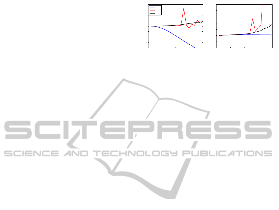
Figure 4: Energy (i.e. the negative log likelihood) vs. time

steps for (left) iteration Type I and (right) iteration Type II

Different colors correspond to different noise levels of the

image sequence.

We use this experiment to test the convergence be-

haviour of algorithms Type I and Type II (see Sec.

3.2). For Type I in some cases we observed an oscil-

lating behavior when nonzero off-diagonal elements

were present in covariance matrix C

(see Fig. 4,

left), which has been our initial motivation to develop

the Type II algorithm. For Type II we always ob-

served rapid convergence (Fig. 4, right), thus for our

other experiments we use Type II only.

Figure 1 shows bias and variance of optical ﬂow

results u

for different noise levels σ. We observe,

that a simple LS estimate (Figure 1a) increasingly un-

derestimates u

for increasing noise, but has a smaller

variance than the other estimators for all noise levels.

The TLS estimator (as used e.g. in (Nestares et al.,

2000; Nestares and Fleet, 2003)) shown in Figure 1b

has much less bias, and also a quite small variance up

to a noise level of 60. However, with further increas-

ing noise, the variance quickly rises, such that results

are completely unreliable. The same is true for the

equilibration method (M

uhlich and Mester, 2004) in

Figure 1c. Its bias is even smaller, but results also be-

come unstable for noise levels higher than 80. The

EIV-ML method is shown in Figure 1d. It features

the same low bias as the equilibration method, but re-

mains much more stable for high noise levels, where

it still shows less bias than the LS approach.

Figure 6 illustrates the distribution on the unit

sphere of estimated ﬂows for the same estimators as in

Fig. 1 for the noise level σ = 90. For the LS estimator

(left) variance of the distribution is almost isotropic

and the maximum biased towards the ’north pole’ of

the sphere, i.e. the point of zero motion. For the TLS

estimator (second left) the distribution becomes a belt

around the sphere. The equilibration method (second

right) results in a somewhat compacter distribution,

not spanning the whole sphere, but becoming wider

across the belt. EIV-ML (right) correctly keeps the

maximum very close to the true value and features

an isotropic distribution with a smaller width than the

equilibration method.

Experiment 3. In a last experiment, we calcu-

20 40 60 80 100 120 140 160 180

100

120

140

160

180

20 40 60 80 100 120 140 160 180

100

120

140

160

180

20 40 60 80 100 120 140 160 180

100

120

140

160

180

Figure 5: Accuracy of optical ﬂow estimates in well struc-

tures areas as classiﬁed by suitably thresholding the esti-

mated CRLB (no ground truth used!). Left to right: Frame

10 of the Ofﬁce sequence, ground truth restricted to image

areas with sufﬁcient image structure, ﬂow estimated using

Sun et al.(Sun et al., 2010), and result using our EIV-ML,

see also Table 1.

late optical ﬂow on the well known Ofﬁce sequence

(Galvin et al., 1998) using our EIV-ML and one of the

best-performing, variational algorithms on the Mid-

dlebury test set

(Baker et al., 2007), i.e. the method

of Sun et al.(Sun et al., 2010). Unlike all measures on

Middlebury, we investigate the performance of the al-

gorithms for well-structured image areas, e.g. for sub-

pixel accurate tracking of well structured but slowly

moving features.

In Fig. 5 resulting ﬂows are shown, restricted to

image areas, where the trace of the estimated covari-

ance matrix of the estimator is below a certain thresh-

old (cmp. with Table 1). We see that ﬂows estimated

by EIV-ML in these areas are closer to the ground

truth than the ones derived by the method of Sun et

al.(Sun et al., 2010).

The average error values (end point error) are

shown in Table 1 for different threshold values ap-

plied to the estimated CRLB. Our approach shows

smaller errors than method (Sun et al., 2010), more

clearly the lower the threshold.

For small thresholds it even shows smaller vari-

ance, which is remarkable, as (Sun et al., 2010) uses

a prior and by this reduces variance at the cost of in-

creased bias. The larger variance of our approach for a

larger thresholds is plausible, as adding a prior biases

Most sequences of the Middlebury test set include large

motions that cannot be handled by a local method without

further means. We thus do not use them here.

VISAPP2014-InternationalConferenceonComputerVisionTheoryandApplications

276

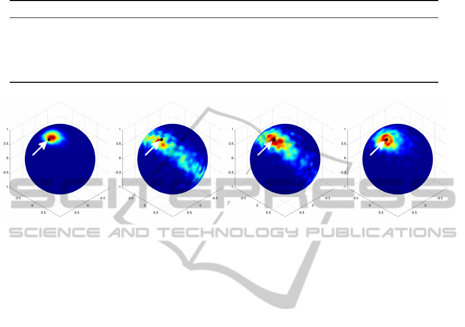
Table 1: Optical ﬂow errors (end point error: mean/variance) on pixels with covariance below the given threshold value for

our approach and Sun et al.(Sun et al., 2010). Density: Percentage of Pixels below Threshold.

Threshold Our Approach Sun et al.(Sun et al., 2010) Density (cmp. (Barron et al., 1994))

0.00001 0.0181 / 0.0620 0.0298 / 0.0697 23.64 %

0.00005 0.0299 / 0.0705 0.0458 / 0.0782 38.53 %

0.0001 0.0397 / 0.0794 0.0559 / 0.0813 48.16 %

0.0005 0.0714 / 0.1224 0.0771 / 0.0821 69.26 %

0.001 0.0844 / 0.1356 0.0867 / 0.0807 78.39 %

Figure 6: Illustration of the distribution of 10

estimated samples for different methods and noise level σ = 90. From left to

right: LS, TLS, equilibration (M

uhlich and Mester, 2004), our approach. The black dot indicates ground truth. We observe

less bias for our method wrt. LS. Lower variance of LS is due to its bias. We further see much less variance compared to TLS

and equilibration.

the result and allows the method to reduce variance.

We conclude that for optical ﬂow our local ap-

proach EIV-ML performs better than an excellent

global algorithm up to a factor of 1.6 in well-

structured image areas.

5 DISCUSSION

Our Type II estimator works ﬁne in cases where we

know that one of the sought parameters in u, say u

, is

certainly nonzero. The problem can then adequately

be described using Cartesian parameters and we can

relate the homogeneous notation to the Cartesian for-

mulation means of w

→ u

. As this transforma-

tion is one-to-one the justiﬁcation of this approach

follows directly from the invariance of the likelihood

under re-parameterizations.

However, for some of the major EIV problems

in computer vision, like e.g. orientation estimation

or projective camera calibration, this is not the case.

There we only know that u lies on the unit sphere.

We cannot set any parameter unequal zero ahead of

time. Unfortunately, the estimation scheme Type I

is not always stable and thus no reliable solution.

What one can do instead, is to exploit that estimat-

ing a point on the unit sphere S

n−1

is equivalent to

estimating a point in the projective space RP

n−1

: A

point u with |u| = 1 represents a direction in R

. Any

other vector r ∈ R

0 which is parallel or antiparal-

lel to u represents the same orientation such that all

vectors in r ∈ R

0 with the same orientation can

be combined into one equivalence class. The set of

all equivalence classes is denoted as the projective

space RP

n−1

= (R

0)/ ∼ with the equivalence re-

lation x ∼ λx, for any λ ∈ R \ 0 and x ∈ R

0. The

so called cell-decomposition property of projective

spaces (cmp. with (Holme, 2010) p.317) states that

each projective space can be decomposed in disjoint

subspaces

n−1

= R

n−1

∪ R

n−2

∪ ...R ∪ R

. (22)

This allows to convert the problem of estimating a

point on the unit sphere S

n−1

(Type I ) to a problem

of estimating a point in n Euclidean spaces. For MAP

estimation, we compute the MAP estimate for each

space and choose the result with the maximum poste-

rior pdf.

To derive the cell-decomposition we assign each

element u ∈ RP

n−1

to the respective subspace R

k−1

iff the last n − k coefﬁcients of u become zero, i.e. we

map u = (u

,. .. ,u

,0, .. ., 0) by

u → (u

,. .. ,u

k−1

) ∈ R

k−1

(23)

for k ∈

{

2,. .. ,n

}

. For k = 1, i.e. u = (u

,0, .. ., 0) we

map u to 1.

Applying our Type II scheme to such problems

by exploiting cell-decomposition is left for future re-

search.

LikelihoodFunctionsforErrors-in-variablesModels-Bias-freeLocalEstimationwithMinimumVariance

277

6 CONCLUSIONS

We introduced a closed form conditional likelihood

function for errors-in-variables problems. It only de-

pends on the parameters of interest, in contrast to

the equivalent likelihood functions as introduced by

Gleser (Gleser, 1981) containing nuisance parame-

ters. Well known estimation schemes known from

literature (Nagel, 1995; Kanatani, 2008; Leedan and

Meer, 2000; Chojnacki et al., 2001; Matei and Meer,

2006) turned out to be special cases of our condi-

tional ML estimator for mutually independent obser-

vations. Therefore error bounds for these estimators

can be calculated as done here. In addition our ap-

proach covers also the case of arbitrary correlations

between measurements.

A straight forward extension of the algorithm from

(Matei and Meer, 2006) iterating SVDs (i.e. Type I )

turned out to have oscillating convergence behavior

when correlated noise is modeled. We did not ob-

serve such behavior for our novel algorithm (i.e. Type

II ). In addition, we experimentally showed for an op-

tical ﬂow application the beneﬁts of having a likeli-

hood function at hand as the likelihood approach dis-

tinguishes good estimates from less reliable estimates.

In such detected, well-structured image regions our

simple local approach even performs better than an

optical ﬂow algorithm with regularization (Sun et al.,

2010) currently among the better performing ones on

the Middlebury test set (Baker et al., 2007). We con-

clude that using a non-regularized estimator can in-

deed be beneﬁcial, when not interested in the whole

image, but the ’good data’ regions. Further we con-

clude that driving regularization by estimated CRLB

may be beneﬁcial and is to be investigated in future

research.

REFERENCES

Abatzoglou, T., Mendel, J., and Harada, G. (1991). The

constrained total least squares technique and its appli-

cations to harmonic superresolution. Signal Process-

ing, IEEE Transactions on, 39(5):1070 –1087.

Andres, B., Kondermann, C., Kondermann, D., K

othe, U.,

Hamprecht, F. A., and Garbe, C. S. (2008). On errors-

in-variables regression with arbitrary covariance and

its application to optical ﬂow estimation. In CVPR.

Baker, S., Roth, S., Scharstein, D., Black, M. J., Lewis, J.,

and Szeliski, R. (2007). A database and evaluation

methodology for optical ﬂow. Computer Vision, IEEE

International Conference on, 0:1–8.

Barron, J. L., Fleet, D. J., and Beauchemin, S. S. (1994).

Performance of optical ﬂow techniques. Int. Journal

of Computer Vision, 12:43–77.

Chojnacki, W., Brooks, M. J., and Hengel, A. V. D. (2001).

Rationalising the renormalisation method of kanatani.

Journal of Mathematical Imaging and Vision, 14:21–

38. 10.1023/A:1008355213497.

Clarke, T. A. and Fryer, J. G. (1998). The Development of

Camera Calibration Methods and Models. The Pho-

togrammetric Record, 16(91):51–66.

Eldar, Y., Ben-Tal, A., and Nemirovski, A. (2005). Ro-

bust mean-squared error estimation in the presence of

model uncertainties. Signal Processing, IEEE Trans-

actions on, 53(1):168 – 181.

Galvin, B., Mccane, B., Novins, K., Mason, D., and Mills,

S. (1998). Recovering motion ﬁelds: An evaluation

of eight optical ﬂow algorithms. In British Machine

Vision Conference, pages 195–204.

Gleser, L. J. (1981). Estimation in a multivariate ”errors

in variables” regression model: Large sample results.

The Annals of Statistics, 9(1):24–44.

Holme, A. (2010). Geometry: Our Cultural Heritage.

Springer, 2 edition.

Huffel, S. V. and Lemmerling, P. (2002). Total Least

Squares and Errors-in-Variables Modeling: Analysis,

Algorithms and Applications. Kluwer Academic Pub-

lishers, Dordrecht, The Netherlands.

Kanatani, K. (2008). Statistical optimization for geomet-

ric ﬁtting: Theoreticalaccuracy bound and high order

error analysis. International Journal of Computer Vi-

sion, 80:167–188. 10.1007/s11263-007-0098-0.

Kelley, C. (1995). Iterative Methods for Linear and Non-

linear Equations. Society for Industrial and Applied

Mathematics, Philadelphia.

Leedan, Y. and Meer, P. (2000). Heteroscedastic regression

in computer vision: Problems with bilinear constraint.

Int. J. of Computer Vision, 2:127–150.

Lemmerling, P., De Moor, B., and Van Huffel, S. (1996).

On the equivalence of constrained total least squares

and structured total least squares. Signal Processing,

IEEE Transactions on, 44(11):2908 –2911.

Lucas, B. and Kanade, T. (August 1981). An iterative im-

age registration technique with an application to stereo

vision. In Proc. Seventh International Joint Conf.

on Artiﬁcial Intelligence, pages 674–679, Vancouver,

Canada.

Markovsky, I. and Huffel, S. V. (2007). Overview

of total least-squares methods. Signal Processing,

87(10):2283 – 2302. Special Section: Total Least

Squares and Errors-in-Variables Modeling.

Matei, B. C. and Meer, P. (2006). Estimation of nonlin-

ear errors-in-variables models for computer vision ap-

plications. IEEE Trans. Pattern Anal. Mach. Intell.,

28:1537–1552.

uhlich, M. and Mester, R. (2004). Unbiased errors-

in-variables estimation using generalized eigensystem

analysis. In ECCV Workshop SMVP, pages 38–49.

Nagel, H.-H. (1995). Optical ﬂow estimation and the

interaction between measurement errors at adjacent

pixel positions. Intern. Journal of Computer Vision,

15:271–288.

Nestares, O. and Fleet, D. (2003). Error-in-variables like-

lihood functions for motion estimation. In Proc. In-

VISAPP2014-InternationalConferenceonComputerVisionTheoryandApplications

278

ternational Conference on Image Processing (ICIP

2003), pages 77–80, Madrid, Spain.

Nestares, O., Fleet, D. J., and Heeger, D. J. (2000). Likeli-

hood functions and conﬁdence bounds for Total Least

Squares Problems. In Proc. IEEE Conf. on Computer

Vision and Pattern Recognition (CVPR’2000), Hilton

Head.

Scharr, H. (2000). Optimal Operators in Digital Image Pro-

cessing. PhD thesis, Interdisciplinary Center for Sci-

entiﬁc Computing, Univ. of Heidelberg.

Simoncelli, E. P. (1993). Distributed Analysis and Repre-

sentation of Visual Motion. PhD thesis, Massachusetts

Institut of Technology, USA.

Sun, D., Roth, S., and Black, M. J. (2010). Secrets of optical

ﬂow estimation and their principles. In CVPR, pages

2432–2439.

Weber, J. and Malik, J. (1995). Robust computation of op-

tical ﬂow in a multi-scale differential framework. In-

ternational Journal of Computer Vision, 14:67–81.

Yeredor, A. (2000). The extended least squares criterion:

minimization algorithms and applications. Signal Pro-

cessing, IEEE Transactions on, 49(1):74 –86.

LikelihoodFunctionsforErrors-in-variablesModels-Bias-freeLocalEstimationwithMinimumVariance

279