
Evaluation of Energy Efficiency of Aggregation in WSNs
using Petri Nets
Ákos Milánkovich, Gergely Ill,
Károly Lendvai, Sándor Imre and Sándor Szabó
Department of Networked Systems and Services, Budapest University of Technology and Economics, Budapest, Hungary
Keywords: Wireless Sensor Networks, Aggregation, Energy Efficiency, FEC, Petri Nets.
Abstract: Energy efficiency is one of the key issues of wireless sensor networks. Aggregation of packets may
increase significantly the lifetime of batteries in exchange for some variations in delay. In this paper we
have investigated how to determine the optimal amount of packets gathered for aggregation that minimizes
the energy consumption of the whole multi-hop network assuming predefined boundary conditions for the
delay. To achieve this goal, appropriate models were created to calculate the energy consumption and delay,
where we exploited the modelling capabilities of generalized stochastic Petri nets. Using these models, the
impact of aggregation was analysed for various test cases. We examined how a network behaves in case of
ideal, low and high BERs and investigated how different FEC coding schemes influence the energy
consumption. Based on these results, we evaluated the properties of aggregation. We will show, that in case
of a good quality radio channel (with low BER) it is not recommended to use FEC codes to optimize for
energy consumption. In case of high aggregation numbers and high BER without the use of FEC the
consumed energy converges to infinity. The simulation results show that using the delay as a constraint can
narrow down the search for the minimal energy consumption of aggregation number vectors.
1 INTRODUCTION
Sensor networks and their applications are getting an
increasingly important role in everyday life. With
their help, we can solve various challenges, such as
the development of agricultural monitoring and
smart metering systems. In these systems, the
devices used as nodes often operate in small-scale
energy source (e.g., alkaline cell, battery). As a
result, during the development of such systems
energy efficient operation is extremely important.
In addition, unlike traditional protocols used in
the Internet, the protocols used in sensor networks
are not particularly sensitive to latency, because in
the vast majority of cases, it is irrelevant when the
data arrives within a certain time T interval to the
data centre. This fact allows the devices to build up
measurement or other useful information, and not
send them immediately, but with some delay, treated
in larger units. Exploiting this, the majority of the
headers of the packets brought together can be
saved, and only appear once in a larger sized packet.
Therefore, the number of bits sent is reduced, which
entails energy saving for the complete network.
To model the behaviour of a complete multi-hop
network, first a model of a chain can be constructed,
which can be extended to an arbitrary network
topology. Using the model presented in this paper,
the aggregation number vector can be determined
solving an optimization problem, which minimizes
energy consumption in the network.
The structure of this paper is the following:
Section 2 presents some related studies; Section 3
introduces the mathematical model based on Petri
nets. In Section 4 the model for energy consumption
is constructed and the methods used for the
simulations are described. Section 5 shows and
analyses the results, and finally, Section 7 concludes
the observations.
2 RELATED WORK
In our previous work (Lendvai et al., 2012), we have
analysed the optimal packet size for energy efficient
communication in delay-tolerant sensor networks
using aggregation of the payload and considering the
SNR (Signal to Noise Ratio) and BER (Bit Error
289
Milánkovich Á., Ill G., Lendvai K., Imre S. and Szabó S..
Evaluation of Energy Efficiency of Aggregation in WSNs using Petri Nets.
DOI: 10.5220/0004668402890297
In Proceedings of the 3rd International Conference on Sensor Networks (SENSORNETS-2014), pages 289-297
ISBN: 978-989-758-001-7
Copyright
c
2014 SCITEPRESS (Science and Technology Publications, Lda.)

Rate) of the channel. In our following work
(Lendvai et al., 2013), we extended our results for a
FEC (Forward Error Correction) enabled channel.
Other studies introduced some other aspects of
aggregation. For example, in (Feng et al., 2011)
some methods can be found on how to avoid data
loss in case of faults in the aggregation tree. The
amendment scheme includes localized aggregation
tree repairing algorithms and distributed
rescheduling algorithms. Yu et al. (Yu et al., 2011)
investigated the security aspects of aggregation by
detecting false temporal variation patterns.
Compared with the existing schemes, the scheme
decreases the communication cost by checking only
a small part of aggregation results to verify the
correctness in a time window. Shoaib and Song
(Shoaib and Song, 2012) deals with particle swarm
optimization (PSO) used to optimize process of
multi-objective data aggregation in vehicular ad-hoc
network.
In this paper, we focus on aggregation without
modifying the data itself; instead, we use bulk
sending and analyse its energy efficiency.
3 PETRI NETS
This section describes the mathematical
representation of Petri nets, which will be used in
our model construction.
The simple Petri net (Peterson, 1981) is a
directed, weighted bipartite graph. The elements of
one vertex class is called Places (P) and the other
class is called Transitions (T). In the directed graph,
all edges connect a place and a transition. A positive
integer, which is called the edge weight is assigned
to the edges. The state of a Petri net can be described
by a function that assigns a non-negative integer to
each place. This is called token distribution, and the
numbers represent the number of tokens at the
places. Formally a Petri net is a ,,,
structure, where
,
,...,
is the finite set of places,
,
,...,
is the finite set of
transitions,
⊆∪ is the set of edges,
and
:→
is the weight function.
3.1 Stochastic Petri Nets (SPN)
The SPN (Marsan, 1990) is a simple extension of
Petri nets. A random firing time (delay) is assigned
to transitions, which can be characterized by
negative exponential probability distribution
function. In addition, the firing semantics is altered
as follows:
A transition can fire at time , if
it became enabled in time
delay was drawn according to the
corresponding distribution function
it has been enabled during , time
interval
The transitions have a unique parameter, called
rate. The
∈
rate is the parameter of a
transition’s delay’s negative exponential
distribution. Such transitions are graphically marked
by empty rectangles opposed to the general,
immediately firing transitions. The drawn
delay
times are formulated as:
1
Next, let us discuss what happens if more than
one transition is enabled as well. In this case, the
firing transition will be the one, who’s drawn time
delay expires first, therefore the enabled transitions
are competing and the decision is based on
probability. After one of the enabled transitions
fired, a new marking is formed. In this case, the
question may arise, should we to draw a new delay
value. There are two possible solutions: a new draw
can be made, or we use the remaining delay values.
The solutions are indifferent, as the delay time has
exponential distribution and the Markov property
(Durrett, 2010) holds. As a result the remaining
firing time is statistically independent of the elapsed
time since the transition became enabled. In
addition, for the enabled transitions the remaining
firing time remains exponentially distributed, no
matter how long they have been enabled.
The generalized stochastic Petri nets (GSPN)
(M.Ajmone Marsan, 1995)are the extensions of
stochastic Petri nets. The GSPN contains the
following enhancements compared to the SPN:
immediate firing transitions (dealing with
logical dependencies),
priorities between transitions,
inhibitor edges
and guard conditions.
4 MODELING AND SIMULATION
In this section first the model for energy
consumption is constructed using Petri nets. Then
the methods and software used for the simulations
are described. The section introduces the analysed
FEC codes and a method for delay calculation.
SENSORNETS2014-InternationalConferenceonSensorNetworks
290

4.1 Energy Consumption Model
To determine the energy consumption, the modelling
power of GSPN-s was used, which can describe the
overall network behaviour. The model developed by
the authors the Places in the Petri net represent the
packet storage queues of the nodes, while
Transitions simulate the sending of packets. During
the creation of the model, we assumed that each
node spends zero time for processing packets. In
addition, the nodes send the aggregated packet
immediately, when they collected as many packets
as their specific aggregation number. In addition,
each node generates packets itself, generated
according to an exponential distribution. According
to previous description, the transitions either have an
exponential delay, or fire immediately. We also
assumed, that the nodes in the network are possess
the same parameters, so the network is
homogeneous. The weight of the edges in the graph
created by the model is the same as the actual node’s
aggregation number, with the default of one.
The developed model actually describes a single
chain network topology. This is sufficient, because
in any network topology a route is required in order
to achieve communication between two nodes,
which route consists of a chain of nodes.
To illustrate our model, let us take a chain
topology consisting of five nodes. Consequently,
assume, that the sensor data reaches the data centre
(sink) in five hops. The graphical appearance of the
model can be seen in Figure 1.
In Figure 1, the nodes of the network are marked
by different colours. It can be seen, that apart from
the first node and the data collector unit (called
sink), all the other nodes are composed of two parts.
The first part consists of the places and transitions
responsible for the data coming from the node’s own
sensors. The second group represents the data
coming from the previous node. The own arrivals
(i.e. the measured values read from the local
sensors) are modelled by transitions with
exponential distribution, which are illustrated by
rectangles containing ‘T’. The arrival of the
neighbour nodes is represented by the immediately
firing transitions. The other transitions of the nodes
immediately fire, when the predefined number of
tokens is available.
The vector of aggregation numbers required to
achieve minimum power consumption of the chain
can be calculated with the previously presented
model. To determine how much energy consumption
a combination of aggregation numbers represent for
the entire chain topology, we have to calculate the
stationary distribution of the system, i.e., the amount
of packets sent to each node in percentage
distribution. Using this result, we can determine the
total power consumption of the chain, if the energy
consumption parameters of the nodes are known.
4.2 PetriDotNet
PetriDotNet (PetriDotNet, 2011) is a software, that
runs on Windows and Mac OS X with a graphical
user interface and can be used for editing, simulate
and analyse Petri nets.
The software was developed by the Department
of Measurement and Information Systems of BUTE.
It was created with the aim of being easy to use in
education. Their aim is to implement the latest
verification and model checking algorithms for this
easily extendable framework, and make it available
to a larger user community. The program is able to:
Saturation-based symbolic state-space
generation, representation, and fixed-point
computation based CTL model checking
Transform the model checking problem to a
linear programming task making it capable of
examining infinite state space Petri nets
Management and analysis of complex data
structures is under development. The program is
able to determine the long-term behaviour of Petri
nets with its "Large Scale Statistics" module. The
user can view the percentage distribution of the
firing of transitions.
4.3 Simulation of Energy Consumption
The determination of the equilibrium distribution
was carried out by the previously presented
PetriDotNet software, because according to our
tests, it was the fastest and it generated the best
output results. To determine the optimal aggregation
number vector, a preparation was needed, so that
PetriDotNet calculates the long-term behaviour of
the appropriate Petri net. This task was performed by
Matlab (Mathworks, 2013).
As shown in
Figure 2, MATLAB was used to
generate all possible permutations of the aggregation
number vector and the associated .pnml Petri net
descriptions. Matlab sequentially calls (can be
parallel) the PetriDotNet software with different
aggregation number combinations. The PetriDotNet
software’s Large Scale Statistics module was used to
simulate 1,000,000 firings to determine the long-
term behaviour. Using the output of the application
and a predefined consumption function was given to
calculate the total consumption of the chain. The
developed consumption function in case of one
EvaluationofEnergyEfficiencyofAggregationinWSNsusingPetriNets
291
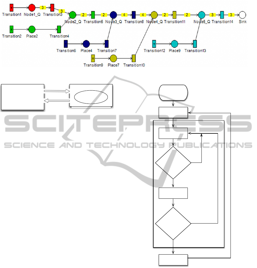
Figure 1: Petri net representation of the problem.
Figure 2: System model.
package is submitted (fire), for a single node in ideal
case (when the radio channel is perfect), is
(Milánkovich et al., 2012):
(1)
In a real system to solve the multi-variable
equation the values of
,
,
,, parameters
have to be defined according to (Milánkovich et al.,
2012). Among these parameters
,
,
describe
the used hardware and , are protocol specific.
The amount of overhead, and the payload and
the size of the ACK is needed to be known. The
formula described above, is a general solution to
calculate the energy consumption, and can be
applied to arbitrary hardware and communication
protocol.
Using formula (1) the energy usage of the whole
chain is the following:
(2)
, where N the length of the aggregation chain and
ϕ
denotes the amount of packets sent (firings in the
model) for the ith node.
4.4 Simulation of Delay
PetriDotNet has been used for calculating the
equilibrium distribution, but could not be used to
determine the amount of delay. To solve this
problem, we created a simulation written in C++.
The implemented program works according to the
algorithm shown in Figure 3.
Initially, the aggregation number permutations,
which were generated previously by Matlab have to
be read. Then cyclically we do the following: the
Figure 3: Flow chart of delay calculation algorithm.
nodes are matched with their corresponding
aggregation number of the current scenario. Then,
aggregated messages are sent to the next neighbours
in the chain in case the number of packets reached
the aggregation number. The sending time of the
messages is recorded, and the simulation goes, until
the iteration number is reached. By the last message
sending the total delay of the chain can be
determined, and saved. Then the next scenario for
aggregation vector is evaluated.
All the nodes aggregate their messages in a
MATLAB
- generate permutations
- generate .pnml
- launch PetriDotNet
- process results
PetriDotNet
Large Scale
Statistics Module
For every node
MATLAB
Read
Permutations
Can we
aggregate ?
Send packet
Is iteration
over?
Save
Results
Own
Arrivals
Y
N
N
Y
SENSORNETS2014-InternationalConferenceonSensorNetworks
292

specific recurring pattern. The length of these
sequences depends on how many nodes preceded the
current node and how many messages were
aggregated by the previous nodes and the current
one. In these sequences it can happen, that the
amount of received messages reach the amount of
the aggregation number, in this case the nodes send
the messages immediately. However, it can also
occur, that the nodes have to wait for more messages
from their previous neighbour to reach their
aggregation number and send the aggregated
messages to the next node. Considering this fact, the
delay fluctuates periodically. These fluctuations can
be summed throughout the entire chain, and exert
synergistic or antagonistic effects.
Given by the consumption formula described
above (2), results on delay by the simulation
algorithm, and binding it with the aggregation
numbers, the best (minimal energy consuming)
aggregation number configuration can be determined
under the given boundary conditions.
4.5 Using FEC
In this section, we examine how the system behaves
in the presence of packet loss (including packet
errors can not be corrected) and FEC (Forward Error
Correction) coding. We examined the energy
consumption of the entire network and the amount
of delay under these conditions. In this analysis, we
need to introduce a new variable, which is denoted
by
. This variable shows how much energy is
needed to encode one bit with FEC codes. The
values and other attributes of the applied FEC
schemes are summarized in Table 1. The values
were determined according to (Lendvai et al., 2013).
In this paper the following block codes were
chosen for analysis: Hamming (255,247) (Lin,
2004), Reed-Solomon (511,501) (Bhargava, 1999),
and BCH (511,502) (Ray-Chaudhuri, 1960), where
the first number represents the output block length
and the second number refers to the input length of
the block code.
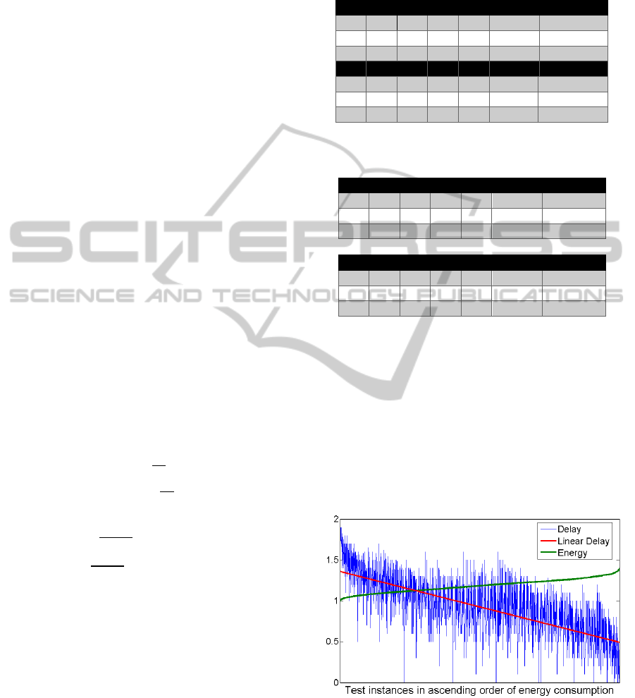
Table 1: Properties of applied FEC codes.
FEC Complexity Type Correctable bits (t)
Hamming
(255,247)
low block 1
5.0522∙10
ReedSolomon
(511,501)
high block 5
5.4344∙10
BCH
(511,502)
high block 4
9.0037∙10
Based on the previous facts (Peterson, 1981), the
formula of energy consumption for sending ad
receiving a packet between two nodes is changed
compared to formula (1) described in the previous
chapter:
(3)
, where is the output of the FEC encoder used,
and is the length in bits of the useful portion of
the FEC code. Other symbols used in the formula (3)
are identical to those presented in section 4.3. If the
values of and are both set to one and
is set to
zero, then the result is the same as if no FEC was
applied.
The packets sent over the noisy radio channel
arrive erroneously at the receiver side. The rate of
errors is expressed by the BER (Bit Error Rate),
which is the number of bit errors divided by the
number the total sent bits. The FEC codes are able to
repair the errors to a certain extent, so that the
package can be restored. The value of PER (Packet
Error Rate) is the probability of failure of a package.
The use of FEC codes reduce the probability of
PER.
Of course, this probability depends on the error
correction capability of the applied FEC code and
the BER of the channel. The following computations
use the value of PER, which is defined by BER
using the following equation:
PER
FEC
=1- 1
1
(4)
, where denotes the error correcting capability of
the FEC, and is the BER.
The formula (5) and (6) jointly determines how
many packets needed to be sent and re-sent in total
for a successful reception. The m in the formula in
the total number of packets we want to send and Φ
specifies how many packets are actually sent for the
successful reception of m packets.
:PER
FEC
1,∈
(5)
PER
FEC
(6)
With formulas (5) and (6), the total consumption of
the chain topology can be determined, which is as
follows:
(7)
EvaluationofEnergyEfficiencyofAggregationinWSNsusingPetriNets
293
, where in this case marks the number of nodes in
the chain.
The presence of packet loss and the use of FEC
affects the delays occur on the chain. Let us imagine
that one node in the chain has incorrectly received
an aggregated packet and was not able to restore it.
Then it cannot send a positive acknowledgment to
the node in before of it, so the previous node
retransmits the packet when its timer expires. The
probability of receiving the packet incorrectly
repeatedly will be less and less, so it will eventually
become a successful reception. Delay suffered
because of faulty reception and retransmission due
to specific boundary conditions is negligible, even if
packet loss occurs in the chain repeatedly.
5 RESULTS
In this section, we report and analyse the results
obtained by simulations with the developed model
with different parameters. To determine the energy
consumption, a sensor network protocol developed
by the authors was used. The calculation method of
the parameters can be found in (Lendvai et al.,
2013). The parameters of the used devices (TI
CC1101 (Texas Instruments, 2011) radio module,
and Atmel AVR XMEGA A3 (Atmel corporation,
2010) microcontroller) are determined by their
datasheets; therefore, the values of the constants in
the formula are the following:
2.339∙10
,
13.742∙10
,
93.387∙10
,
288
,
80
.
During the simulations, we have investigated the
five-node-long chain shown in Figure 1.
In the simulations, the delays are in the order of
hours, because the delay resulting of the additional
packet loss – at worst a few minutes – is considered
negligible.
The following section describes various test
cases. Table 2 and Table 3 presents the first and last
three of aggregation number vectors in case we
optimised for energy efficiency. Table 3 shows the
corresponding aggregation numbers of the cases
with the most and least delays. In these scenarios,
the radio channel was considered ideal (i.e. causing
no bit errors). The columns N1-N5 represent the
aggregation numbers on the nodes of the chain.
Table 2: The aggregation numbers of the best and worst
energy consumption.
N1 N2 N3 N4 N5 E [J] Delay [h]
5 5 5 5 5 427.02 2
4 5 5 5 5 428.43 1.9
5 4 5 5 5 429.83 1.9
N1 N2 N3 N4 N5 E [J] Delay [h]
1 1 1 1 1 597,5 0
2 1 1 1 1 594,2 0,1
3 1 1 1 1 592,2 0,1998
Table 3: Aggregation numbers of the best and worst
delays.
N1 N2 N3 N4 N5
E [J]
Delay [h]
1 2 3 4 5 475,6 0
1 2 3 2 5 495,02 0
1 1 3 4 5 495,02 0
N1 N2 N3 N4 N5 E [J] Delay [h]
5 5 5 5 5 427,02 2
4 5 5 5 5 428,43 1,9
5 4 5 5 5 429,83 1,9
Figure 4 and Figure 5 show the diagrams of the
simulation results of scenarios with no bit errors on
the radio channel. The values of energy consumption
have been scaled so that they can be displayed on a
common chart with the values of delay. The
simulations inspected a five-node-long chain, where
the aggregation numbers were integers between zero
and five, which equals the inspection of 3125 test
cases. To help the interpretation of the presented
charts, the linear regression of the delay is also
drawn.
Figure 4: The characteristics of energy consumption and
delay of various aggregation vectors in ascending order of
energy consumption.
The values of Figure 4 are the scenarios of
aggregation number vectors in ascending order of
energy consumption, while the values of Figure 5
SENSORNETS2014-InternationalConferenceonSensorNetworks
294
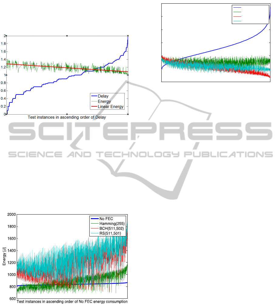
are shown in ascending order of delay. In terms of
energy efficiency the aggregation number vector
(5,5,5,5,5) performed best, however, in terms of
delay the best vector was (1,1,1,1,1).
Figure 5: The characteristics of energy consumption and
delay of various aggregation vectors in ascending order of
delay.
The simulations of Figure 6 were conducted on a
homogeneous radio channel with a BER value of
5∙10
for every link. The used aggregation
numbers were low integers between zero and five. It
can be seen, that FEC schemes cause additional
energy consumption compared to baseline. Among
FEC schemes, the ones with longer code length
produce higher consumption values.
Figure 6: Aggregation number vectors in order of energy
consumption without FEC at a homogeneous BER of
5∙10
.
Figure 7 shows the simulation results for energy
consumption without FEC and with some FEC
schemes on a radio channel with homogeneous BER
(5∙10
). This figure shows clearly, that if the
value of BER increases, the importance of FEC
grows in terms of energy efficiency. If BER is
Figure 7: Aggregation number vectors in ascending order
of energy consumption without FEC with homogeneous
BER of 5∙10
.
increased two orders of magnitude, then the
scenarios using FEC produce a much more efficient
result. The diagrams of Figure 7 seem to contradict
the expectations, as the scenarios using FEC do not
follow the trends of the base scenario without FEC.
The aggregation number vectors are low in case
of low energy consumption without FEC when we
simulated on a worse quality radio channel, because
the length of the aggregated packet is less, so that
the PER is also less according to formula (4), which
results in a lower energy consumption. On the
contrary, in case of higher aggregation number
vectors the packets must be resent more frequently
due to packet errors, so the energy consumption
increases. However, in case of using FEC, the higher
aggregation number vectors produce better energy
efficiency (i.e. lower consumption values). This can
be explained as the following: the use of FEC
decreases the PER, so the number of resent packets
also decreases, which results in a lower energy
consumption. The more we aggregate the beneficial
effects of FEC codes increase.
Figure 8 shows the results of a simulation
conducted with a BER value of 5∙10
, and the
aggregation numbers were the permutations of the
following set: 30,21,12,5,10. According to the
charts, the best performing FEC scheme was the
Hamming code.
Figure 9 shows the energy consumption of the
test cases with different aggregation number vectors,
but identical delays (in this case 0.9 hours). It can be
seen, that using the delay, as a boundary condition
there is no exact solution for minimal energy
consumption, because the different aggregation
numbers require different amounts of energy.
Practically the aggregation number vector with the
minimum energy can be selected for a given delay.
2000
4000
6000
8000
10000
12000
14000
Test instances in ascending order of No FEC energy consumption
Energy [J]
No FEC
Hamming (255)
BCH(511,502)
RS(511,501)
EvaluationofEnergyEfficiencyofAggregationinWSNsusingPetriNets
295
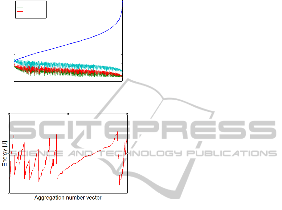
Figure 8: The values of energy consumption for
aggregation number permutations of {30,21,12,5,10} and
BER value of 5∙10
.
Figure 9: Energy consumption of aggregation number
vectors for identical delays (0.9 h).
6 CONCLUSIONS
According to our investigations on packet
aggregation in wireless sensor networks we found,
that in real systems there is a conflict between
energy consumption and delay, therefore finding the
optimal value can be a question of trade-off.
We also concluded, that in case of a good quality
radio channel (with low BER) it is not worthy to use
FEC codes in case optimizing for energy
consumption. The reason is that the additional
energy needed for coding and the overhead of the
code word length is present in the system. On the
contrary, in case of bad quality channels (with
higher BER) the use of FEC is reasonable to
decrease energy consumption as the energy needed
for retransmission due to packet errors can be
spared.
The use of FEC in case of higher BER and
aggregation number vectors is also beneficial,
because the PER of longer packets decreases, which
results in lower energy consumption. The energy
consumption in case of high aggregation numbers
and high BER without the use of FEC converges to
infinity.
The simulation results show that the delay as a
constraint can narrow down the search for the
minimal energy consumption of aggregation number
vectors.
Further research will focus on the application of
the presented model in routing algorithms for sensor
networks.
ACKNOWLEDGEMENTS
This research has been supported by BME-Infokom
Innovátor Nonprofit Ltd., http://www.bme-
infokom.hu.
This research has been sponsored by “Új
Széchenyi Terv” GOP-1.1.1-11-2012-0253,
“Development of new production sampling, data
transmission and evaluation technology, and
operational environment for agricultural holding
sales and organization, - AgroN2”.
REFERENCES
Atmel corporation, 2010. AVR XMEGA A3 Device
Datasheet.
Bhargava, S. B. W. a. V. K., 1999. Reed-Solomon Codes
and Their Applications., Wiley-IEEE Press.
Durrett, R., 2010. Probability: Theory and Examples.
Fourth Edition.
Feng, Y., Tang, S. & Dai, G., 2011. Fault tolerant data
aggregation scheduling with local information in
wireless sensor networks., pp. 453-463.
Lendvai, K., Milankovich, A., Imre, S. & Szabo, S., 2012.
Optimized packet size for energy efficient delay-
tolerant sensor networks. Barcelona, pp. 19-25.
Lendvai, K., Milankovich, A., Imre, S. & Szabo, S., 2013.
Optimized packet size for energy efficient delay-
tolerant sensor networks with FEC. Zagrab.
Lin, D. J. C. S., 2004. Error Control Coding:
Fundamentals and Applications.
M.Ajmone Marsan, G. B. G. C. S. D. a. G. F., 1995.
Modelling with Generalized Stochastic Petri Nets.
John Wiley and Sons.
Marsan, M. A., 1990. Stochastic Petri nets: An elementary
introduction. In: Advances in Petri Nets 1989., pp. 1-
29.
Mathworks, [Online] Available at:
http://www.mathworks.com/products/matlab/
Milánkovich, Á., Lendvai, K., Imre, S. & Szabo, S., 2012.
Radio propagation modeling on 433 MHz. EUNICE
2012, 29 Aug.pp. 1-12.
40
50
60
70
80
90
100
110
120
130
Test instances in acending order of No FEC energy consumption
Energy [J]
No FEC
Hamming (255)
BCH (511,502)
RS (511,501)
SENSORNETS2014-InternationalConferenceonSensorNetworks
296

Peterson, J. L., 1981. Petri Net Theory and the Modeling
of Systems. Prentice Hall.
PetriDotNet, [Online] Available at:
http://www.inf.mit.bme.hu/research/tools/petridotnet.
Ray-Chaudhuri, R. C. B. a. D. K., 1960. Further results on
error correcting binary group codes., pp. 279-290.
Shoaib, M. & Song, W.-C., 2012. Data aggregation for
Vehicular Ad-hoc Network using particle swarm
optimization. Seoul, pp. 1-6.
Texas Instruments, 2011. [Online] Available at:
http://www.ti.com/lit/ds/symlink/cc1101.pdf.
Yu, L., Li, J., Cheng, S. & Xiong, S., 2011. Secure
continuous aggregation via sampling-based
verification in wireless sensor networks. Shanghai, pp.
1763-1771.
EvaluationofEnergyEfficiencyofAggregationinWSNsusingPetriNets
297
