
Image-based Modelling of Ocean Surface Circulation from Satellite
Acquisitions
Dominique B
´
er
´
eziat
1
and Isabelle Herlin
2,3
1
Universit
´
e Pierre et Marie Curie, 4 place Jussieu, 750005, Paris, France
2
Inria, B.P. 105, 78153 Le Chesnay, Paris, France
3
CEREA, Joint Laboratory ENPC - EDF R&D, Universit
´
e Paris-Est, Cit
´
e Descartes Champs-sur-Marne,
77455 Marne la Vall
´
ee Cedex 2, Paris, France
Keywords:
Dynamic Model, Optical Flow, Data Assimilation, Satellite Image, Ocean Circulation.
Abstract:
Satellite image sequences permit to visualise oceans’ surface and their underlying dynamics. Processing these
images is then of major interest in order to better understanding of the observed processes. As demonstrated
by state-of-the-art, image assimilation allows to retrieve surface motion from image sequences, based on
assumptions on the dynamics. In this paper we demonstrate that a simple heuristics, such as the Lagrangian
constancy of velocity, can be used, and successfully replaces the complex physical properties described by the
Navier-Stokes equations, for assessing surface circulation from satellite images. A data assimilation method
is proposed that includes an additional term a(t) to this Lagrangian constancy equation. That term summarises
all physical processes other than advection. A cost function is designed, which quantifies discrepancy between
satellite data and model values. The cost function is minimised by the BFGS solver with a dual method of
data assimilation. The result is the motion field and the additional term a(t). This last component models
the forces, other than advection, that contribute to surface circulation. The approach has been tested on Sea
Surface Temperature of Black Sea. Results are given on four image sequences and compared with state-of-
the-art methods.
1 INTRODUCTION
Satellite image sequences permit to visualise oceans’
surface and their underlying dynamics. Processing
these images is then of major interest in order to better
understanding of the observed processes and forecast
extreme events. As demonstrated by state-of-the-art,
image assimilation allows to retrieve surface motion
from image sequences, using heuristics on the dynam-
ics (Papadakis et al., 2007; Titaud et al., 2010).
Advanced 3D oceanographic models are avail-
able in the literature. These models are based on
Navier-Stokes equations (see for instance the NEMO
model
1
). As satellites nowadays observe the sea sur-
face with a high spatial resolution, it becomes pos-
sible to estimate surface circulation from these data
with a simplified model, such as the shallow water
model (Vallis, 2006). This 2D model has been proven
to be suitable for representing the surface circulation
of closed seas, such as Black Sea (Oguz et al., 1992).
The shallow water equations have also been success-
1
http://www.nemo-ocean.eu/
fully used to estimate the upper layer circulation of
Black Sea from Sea Surface Temperature (SST) im-
ages (Korotaev et al., 2008; Huot et al., 2010) with a
data assimilation method.
In this paper, we propose to learn dynamics
from SST image acquisitions with a data assimila-
tion method applied to an empirical model, derived
from the shallow water equations. This is an image-
based approach to model the surface dynamics. In the
shallow water model, surface circulation is described
by the horizontal velocity, that is advected by itself
and subject to geophysical forces such as Coriolis,
Earth gravity and viscosity. The advection process
is kept in the empirical model, but all non-transport
components are summarised in a global term, denoted
a (letter a stands for additional), that is estimated
by our approach. Adding this term to the advection
one is similar, from a mathematical point of view, to
the weak data assimilation framework (Sasaki, 1970;
Dee, 2005; Tr
´
emolet, 2006; Valur H
´
olm, 2008). Such
data assimilation method is then designed to compute
the solution: a cost function is constructed whose con-
288
Béréziat D. and Herlin I..
Image-based Modelling of Ocean Surface Circulation from Satellite Acquisitions.
DOI: 10.5220/0004669602880295
In Proceedings of the 9th International Conference on Computer Vision Theory and Applications (VISAPP-2014), pages 288-295
ISBN: 978-989-758-009-3
Copyright
c
2014 SCITEPRESS (Science and Technology Publications, Lda.)

trol variables are the motion field at the first acquisi-
tion date and the value of the additional term a(t) at
each date of the acquisition interval. The minimum of
the cost function is obtained thanks to optimal control
techniques (Lions, 1971).
Section 2 provides the notations that are used in
the remaining of this paper and the mathematical de-
scription of the proposed approach in order to model
the dynamics of the ocean’s upper layer. The data
assimilation method is briefly outlined in Section 3.
It corresponds to a weak formulation with a non ad-
vective term in the evolution equation. The imple-
mentation is shortly given in Section 4, in order to
permit that interested Readers apply the method by
themselves. Results on four SST image sequences ac-
quired over Black Sea by NOAA-AVHRR sensors are
displayed and quantified in Section 5.
2 PROBLEM STATEMENT
Image data are acquired on a bounded rectangle of
2
, named Ω, and on a temporal interval [0, T]. Let
define A = Ω × [0,T] the corresponding space-time
domain, on which the dynamics is modelled. A
point x ∈ Ω is defined as x =
x y
T
and the mo-
tion vector at point x and date t ∈ [0,T] is written
w(x,t) =
u(x,t) v(x,t)
T
. At each date t, the mo-
tion field on the domain Ω is written as w(t). N Sea
Surface temperature acquisitions are available at dates
t
i
, i = 1 ···N. They are denoted T (t
i
) with pixels val-
ues T (x,t
i
).
A state vector X is defined on A. It includes the
two components u and v of the motion vector w(x,t)
and a pseudo-temperature value T
s
(x,t), which has
properties similar to those of the Sea Surface Temper-
ature value: X(x,t) =
w(x,t)
T
T
s
(x,t)
T
. At the
end of the data assimilation process, the discrepancy
between the pseudo-temperature and the satellite ac-
quisition values has to be small.
The heuristics on dynamics, used in the paper,
are derived from the shallow water equations, that
express the principles of mass and momentum
conservation. Circulation of the upper ocean is
represented by the 2D velocity w =
u v
T
and
the thickness h of the mixed layer. The sea surface
temperature T
s
is transported by the motion field.
This provides the set of equations:
∂u
∂t
= −u
∂u
∂x
− v
∂u
∂y
+ f v − g
0
∂η
∂x
+ K
w
∆u (1)
∂v
∂t
= −u
∂v
∂x
− v
∂v
∂y
− f u − g
0
∂η
∂y
+ K
w
∆v (2)
∂η
∂t
= −
∂(uη)
∂x
−
∂(vη)
∂y
− h
m
∂u
∂x
+
∂v
∂y
(3)
∂T
s
∂t
= −u
∂T
s
∂x
− v
∂T
s
∂y
+ K
T
∆T
s
(4)
with η the thickness anomaly η = h − h
m
, h
m
the av-
erage value of h, K
T
the temperature diffusion pa-
rameter, f the Coriolis parameter, K
w
the viscosity
and g
0
= g(ρ
0
− ρ
1
)/ρ
0
the reduced gravity. ρ
0
corre-
sponds to the reference density and ρ
1
to the average
density of the mixed layer.
As explained in the introduction, we propose to
group all geophysical forces that do not correspond to
advection in a unique term, named “additional term”
and denoted by a. The variable η is then considered
as an hidden variable of the system and is included in
a. In such way, Eqs. (1),(2),(3) reduce to:
∂u
∂t
= −u
∂u
∂x
− v
∂u
∂y
+ a
u
(5)
∂v
∂t
= −u
∂v
∂x
− v
∂v
∂y
+ a
v
(6)
where a =
a
u
a
v
expresses the discrepancy to the
Lagrangian constancy of velocity:
dw
dt
=
∂w
∂t
+ (w.∇)w = a (7)
From Equations (1,2), we get:
a
u
= f v − g
0
∂η
∂x
+ K
w
∆u (8)
a
v
= − f u − g
0
∂η
∂y
+ K
w
∆v (9)
where η verifies Eq.(3).
Our approach allows to estimate w(0) and the ad-
ditional term a(t) at each date t ∈ [0,T], thanks to a
data assimilation process summarised in Section 3.
Deriving the values a(t) allows to describe empiri-
cally the physical processes producing the image se-
quence.
Eqs. (7) and (4) are further contracted in an evolu-
tion model of the state vector X:
∂X
∂t
+ (X) =
a
0
(10)
An observation equation links the state vector to
the observed Sea Surface Temperature images acqui-
sitions T :
X = T + ε
R
(11)
Image-basedModellingofOceanSurfaceCirculationfromSatelliteAcquisitions
289
The observation operator projects the state vec-
tor into the space of image observations and conse-
quently: X = T
s
. The term ε
R
(x,t) models the ac-
quisition noise and the uncertainty on the state vector
value. This last comes from the approximation of the
model and from the discretization errors.
Some approximate knowledge of the value X(0)
could be available and named background X
b
. How-
ever, the result of the state vector at date 0 is not ex-
actly equal to that background value and a term ε
B
is
therefore introduced:
X(x,0) = X
b
(x) + ε
B
(x) (12)
The variables ε
R
and ε
B
are supposed independent,
unbiased, Gaussian and characterised by their respec-
tive covariance matrices R and B.
Eqs. (10), (11), (12) summarise the whole knowl-
edge that is available to model the surface dynam-
ics. This knowledge is processed by our approach
thanks to a data assimilation algorithm that is shortly
described in Section 3.
3 DATA ASSIMILATION
In the data assimilation scientific community, an
approach named weak 4D-Var has been defined:
in order to obtain the solution X that solves Sys-
tem (10), (11), (12), a cost function is designed, that
is minimised with control on ε
B
and on the values of
the additional term a:
J[ε
B
,a] =
ε
B
,B
−1
ε
B
+
Z
t
γk∇a(t)k
2
+
Z
t
h
X(t) − T (t), R
−1
( X(t) − T (t))
(13)
where
h
·,·
i
denotes the canonical inner product in an
abstract Hilbert space on which the state vector is
defined, with norm k.k
2
and k∇ak
2
=
h
∇a
u
,∇a
u
i
+
h
∇a
v
,∇a
v
i
.
The first term comes from Eq. (12) and expresses
that the value X(0) at date 0 should stay close to the
background value X
b
. The second term constrains
the additional term a(t) to be spatially smooth. The
last term, coming from Eq. (11), expresses that the
pseudo-temperature value T
s
has to be close to that
of satellite acquisitions at the end of the assimilation
process.
The gradient of J is derived with calculus of vari-
ation (Lions, 1971). Its two components are:
∂J
∂ε
B
[ε
B
,a] = 2
B
−1
ε
B
+ λ(0)
(14)
∂J
∂a(t)
[ε
B
,a] = 2 (−γ∆a(t) + λ(t)) (15)
with λ(t) being the adjoint variable, that is computed
backward with the two following equations:
λ(T) = 0 (16a)
−
∂λ
∂t
+
∂
∂X
∗
λ =
T
R
−1
( X − T ) (16b)
The adjoint operator
∂
∂X
∗
is defined by:
h
Zη,λ
i
=
h
η,Z
∗
λ
i
. (17)
Proof: For sake of simplicity, we suppose in this
proof that Eq. (10) is written as
∂X
∂t
+ (X) = a.
The state vector and the functional J depend on ε
B
and a(t). Let δJ and δX be the perturbations on J and
X obtained if ε
B
and a(t) are respectively perturbed
by δε
B
and δa(t).
From the definition of δJ, we obtain:
δJ = 2
δε
B
,B
−1
ε
B
+ 2
Z
t
(γ
h
∇δa(t), ∇a(t)
i
)
+2
Z
t
δX(t),
T
R
−1
[ X(t) − T (t)]
(18)
The evolution equation of X, Eq. (10), gives:
∂δX(t)
∂t
+
∂
∂X
δX(t) = δa(t) (19)
and that of background, Eq. (12):
δX(0) = δε
B
(20)
Eq. (19) gives, after multiplication by λ(t) and
integration on the space-time domain, the following
equality:
Z
t
∂δX(t)
∂t
,λ(t)
+
Z
t
∂
∂X
δX(t), λ(t)
=
Z
t
h
δa(t), λ(t)
i
(21)
Integration by parts is applied on the first term and
the adjoint operator is used in the second one in order
to obtain:
h
δX(T ),λ(T )
i
−
h
δX(0),λ(0)
i
+
−
Z
t
δX(t),
∂λ(t)
∂t
+
Z
t
δX(t),
∂
∂X
∗
λ(t)
=
Z
t
h
δa(t), λ(t)
i
(22)
From Eq.(16a), it comes that
h
δX(T ),λ(T )
i
has a null
value. From Eq. (20) it comes that
h
δX(0),λ(0)
i
is
equal to
h
δε
B
,λ(0)
i
. Eq. (16b) is then used to obtain:
−
δX(t),
∂λ(t)
∂t
+
δX(t),
∂
∂X
∗
λ(t)
=
δX(t),
T
R
−1
( X(t) − T (t))
(23)
VISAPP2014-InternationalConferenceonComputerVisionTheoryandApplications
290

and rewrite Eq. (22) as:
Z
t
δX(t),
T
R
−1
( X(t) − T (t))
=
h
δε
B
,λ(0)
i
+
Z
t
h
δa(t), λ(t)
i
(24)
From this and Eq. (18), we derive:
δJ =2
δε
B
,B
−1
ε
B
− 2
Z
t
γ
h
δa(t), ∆a(t)
i
+
2
h
δε
B
,λ(0)
i
+ 2
Z
t
h
δa(t)λ(t)
i
(25)
and obtain the gradient of J, as written in Eqs. (14,15).
The cost function J is minimised with an iterative
steepest descent method. At each iteration, the for-
ward time integration of X is performed, according to
Eq. (10). This forward integration provides the value
of J. Then a backward integration of λ, according to
Eqs. (16a) and (16b), computes the value of ∇J. An
efficient solver (Byrd et al., 1995) is used to perform
the optimisation given values of J and ∇J. (Le Dimet
and Talagrand, 1986) is the first paper of the literature
that describes the use of such method for estimating
the initial state vector value.
4 NUMERICAL
IMPLEMENTATION
Time integration of Eq. (10) relies on an explicit Euler
scheme. Space discretization of motion advection:
∂u
∂t
+ u
∂u
∂x
+ v
∂u
∂y
= 0 (26)
∂v
∂t
+ u
∂v
∂x
+ v
∂v
∂y
= 0 (27)
involves a source splitting method (Wolke and Knoth,
2000), that is explained below.
Given an integration interval [t
1
,t
2
], Eqs. (28)
and (29) are first independently integrated:
∂u
a
∂t
+ u
a
∂u
a
∂x
= 0 t ∈ [t
1
,t
2
] (28)
∂u
b
∂t
+ v
∂u
b
∂y
= 0 t ∈ [t
1
,t
2
] (29)
with u
a
(x,y,t
1
) = u
b
(x,y,t
1
) = u(x,y,t
1
). Then
u(x,y,t
2
) is obtained as u(x,y,t
2
) = u
b
(x,y,t
2
) +
u
a
(x,y,t
2
) − u(x,y,t
1
).
The linear advection of Eq. (29) is approxi-
mated by a first-order upwind scheme, as described
in (Hundsdorfer and Spee, 1995). The nonlinear ad-
vection of Eq. (28) is first rewritten in a conservative
form:
∂u
∂t
+
∂
∂x
1
2
u
2
= 0 (30)
and approximated by a first-order Godunov
scheme (LeVeque, 1992).
The backward time integration of the adjoint vari-
able λ involves the adjoint operator
∂
∂X
∗
(see
Eq. (16b)). In order to be accurate, the method re-
quires the adjoint of the discrete model and not the
discretization of the continuous adjoint. The discrete
adjoint operator
∂
∂X
∗
is then obtained with the au-
tomatic differentiation software Tapenade (Hasco
¨
et
and Pascual, 2004; Hasco
¨
et and Pascual, 2013).
The background used in Eq. (12) is defined as null
for motion and as the first image of the studied se-
quence for the pseudo-temperature.
5 RESULTS
For sake of simplicity, we name in the following EM,
or Empirical Model, the dynamic model described in
Sections 2 and 3: it includes the advection model and
the additional term summarising the Coriolis, gravity
and viscosity forces.
The proposed method has been experimented on
several Sea Surface Temperature (SST) sequences,
acquired over Black Sea by NOAA-AVHRR sensors,
and results are given for four of them in this paper.
First, we discuss the ability of the proposed
method to correctly estimate motion. For that pur-
pose, EM results are compared with those obtained
by one of the best optical flow method (Sun et al.,
2010) of the literature. The satellite sequence is dis-
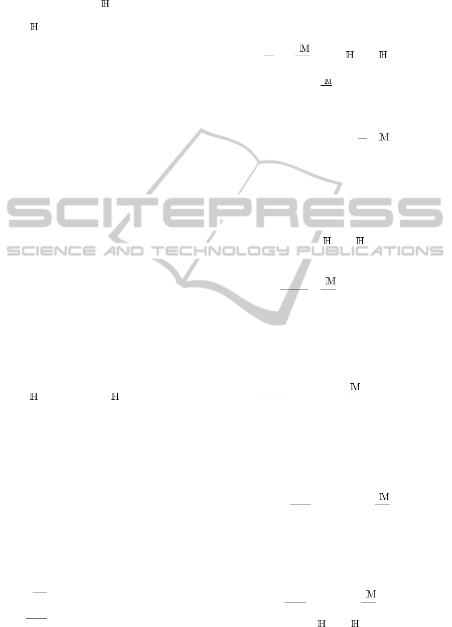
played on Figure 1. Acquisition dates are at 30 min,
6 hours, 15 hours, and 30 hours after the beginning of
the studied temporal interval.
Two gyres are clearly visible on these data. Mo-
tion results w(0), obtained by (Sun et al., 2010) and
EM, are displayed on Figure 2. EM successes to cap-
ture the two gyre structures while Sun et al. fails. As
w(0) is obtained from the analysis of the whole image
sequence, its correct estimation means that the phys-
ical processes involved in a(t) are correctly assessed
by the empirical model. It means that the geophysical
non advective forces may be described as a whole in
a unique term a(t).
Second, we examine the capability of EM to track
features or points of interest on the whole image se-
quence. An accurate tracking result means that mo-
tion estimated by EM is correct on the studied tempo-
ral interval and properly transports image structures.
A sequence of four SST images acquired in October
8
th
2005 is displayed on Figure 3. Acquisition dates
are at 30 min, 10 hours 15 min, 12 hours, 15 hours 30
min, after the beginning of the studied interval. Nine
Image-basedModellingofOceanSurfaceCirculationfromSatelliteAcquisitions
291
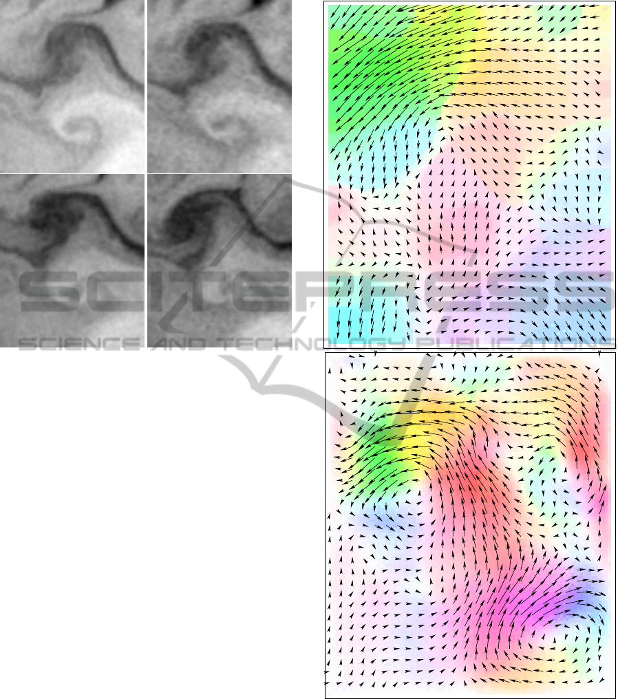
Figure 1: Top to bottom, left to right: SST images acquired
on October 10
th
2007, over Black Sea.
characteristic points are defined in white on the first
observation. Points are surrounded by a coloured cir-
cle that helps to discriminate them on the following
observations. These points are considered as charac-
teristic, because they sample the various types of tra-
jectories that can be observed on the sequence. On
observations 2 to 4, the position of these nine points
obtained with Sun’s method are in red while those ob-
tained with EM are in blue. On the fourth acquisition,
in the “light pink circle” on the upper right, the point
obtained with Sun’s optical flow is outside of the im-
age domain. Looking at the trajectories, it can be ob-
served that Sun’s algorithm fails to track these char-
acteristic points, due to a wrong estimation of motion.
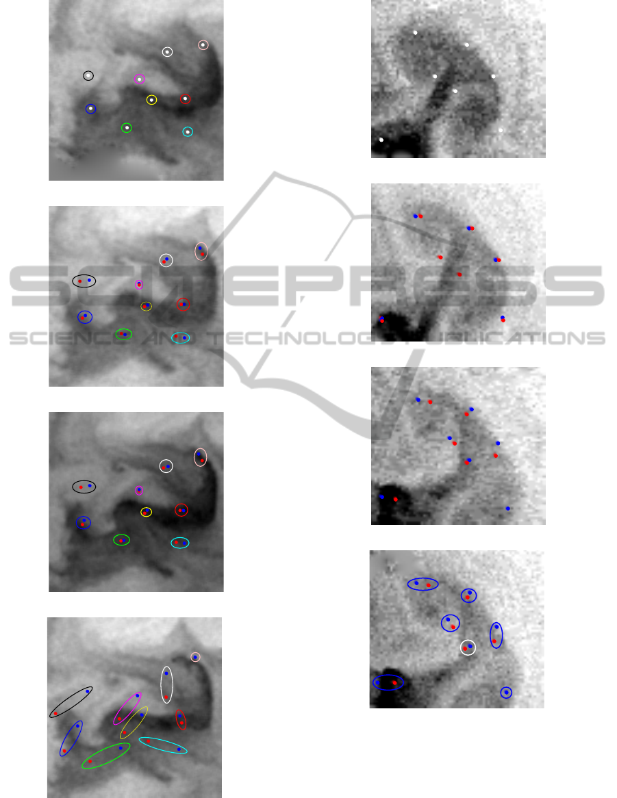
Another sequence of five SST images, acquired in
July 2007 is displayed on Figure 4. Acquisition dates
are at 30 min, 8 hours 15 min, 13 hours, 22 hours 30
min, 24 hours 30 min from the beginning of the stud-
ied interval. Seven characteristic points are defined
in white on the first observation. Points positions ob-
tained with Sun’s optical flow are in red while those
obtained with EM are in blue. At the second date,
two points are at the same position with Sun’s method
and EM: only the red point is visible as the blue one
is hidden behind it. On the fourth observation, one
red point has disappeared as it is located outside of
the image domain. On the last image, the colour of
the ellipse surrounding each set of points gives an
additional information on the quality of the result: a
Figure 2: Motion results computed by Sun (up) and EM
(down) at first observation date. The arrow representation
is superposed to the coloured one.
blue ellipse means that our method gives the best re-
sult, while the white one means that both methods are
equivalent.
Again, Sun’s motion results fail to track character-
istic points on these data as physical processes are not
correctly assessed.
VISAPP2014-InternationalConferenceonComputerVisionTheoryandApplications
292
(a) Observation 1
(b) Observation 2
(c) Observation 3
(d) Observation 4
Figure 3: Tracking of characteristic points. Sun’s algorithm
in red, EM in blue.
(a) Observation 1
(b) Observation 2
(c) Observation 4
(d) Observation 5
Figure 4: Tracking of characteristic points. A blue ellipse
on (d) expresses that EM is the best while the white ellipse
expresses that results are equivalent.
Last, EM is also compared with the optical flow
estimation of Suter (Suter, 1994), that is dedicated to
fluid flows. The SST sequence was acquired in May
14
th
2005 and contains five observations at 30 min, 2
Image-basedModellingofOceanSurfaceCirculationfromSatelliteAcquisitions
293
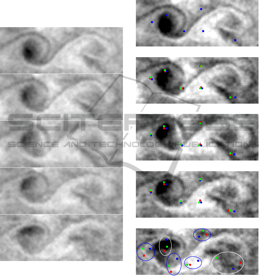
hours and 45 min, 5 hours and 15 min, 7 hours and 15
min, 16 hours and 15 min after the beginning of the
studied interval. They are displayed on Figure 5.
Figure 5: Five consecutive observations of the sequence ac-
quired in May 14
th
2005.
As previously, six feature points are chosen on the
first observation and displayed on the upper image of
Figure 6. Their final position on the fifth observation
is given in the lower part of the same figure.
Suter’s and Sun’s methods being based on vari-
ational optical flow approaches, they are only con-
strained by grey level values and not by the under-
lying dynamics. However, Suter’s algorithm provides
better result than Sun’s method, because it is specif-
ically designed for fluid flows motion. In particular,
it can correctly assess rotational motion. From left to
right in Subfigure 6(e): EM gives the best result for
(a) Characteristic points on the first observation.
(b) On second one.
(c) On third one.
(d) On fourth one.
(e) Characteristic points on the last observation.
Figure 6: Tracking of feature points displayed in blue in (a).
Sun’s result is in red, Suter’s in green and EM’s in blue.
the first, third, fourth and fifth points (blue ellipses).
For the second and sixth (white ellipses) points, it is
not possible to determine which one from Suter’s al-
gorithm and EM provides the best result.
The same conclusion is valid for all studied image
sequences.
VISAPP2014-InternationalConferenceonComputerVisionTheoryandApplications
294

6 CONCLUSIONS
This paper describes how to learn the ocean surface
dynamics from an empirical model, EM, that sum-
marises the shallow water equations by an advec-
tion term and an additional term a. This last repre-
sents physical processes such as the Coriolis force,
the gravity force and the viscosity. A data assimila-
tion algorithm is defined for EM that estimates the
velocity field at the first acquisition date and the ad-
ditional term a(t) at each date of the studied inter-
val. a(t) is of major importance for correctly assess-
ing the hidden physical processes and accurately es-
timating motion on the whole image sequence. The
algorithm does not involve any parameter other than
those of the data assimilation framework (error co-
variance matrices). The method has been illustrated
on several SST sequences of Black Sea and has been
quantified by tracking feature points. Moreover, it has
been compared with state-of-the-art optical flow algo-
rithms. The conclusion is that a model of dynamics,
even if simple, improves motion estimation and al-
lows tracking of structures.
This approach may be seen as a first step to model
the physical processes occurring at the ocean surface
from image data. The short-term perspectives will be
to compare the additional term a(t) with forces in-
volved in the shallow water model, in order to further
validate the ability of the empirical model to assess
geophysical processes.
ACKNOWLEDGEMENTS
Data have been provided by E. Plotnikov and G. Ko-
rotaev from the Marine Hydrophysical Institute of
Sevastopol, Ukraine.
REFERENCES
Byrd, R. H., Lu, P., and Nocedal, J. (1995). A limited
memory algorithm for bound constrained optimiza-
tion. Journal on Scientific and Statistical Computing,
16(5):1190–1208.
Dee, D. (2005). Bias and data assimilation. Quaterly Jour-
nal of the Royal Meteorological Society, 131:3323–
3343.
Hasco
¨
et, L. and Pascual, V. (2004). Tapenade 2.1 user’s
guide. Technical Report 0300, INRIA.
Hasco
¨
et, L. and Pascual, V. (2013). The Tapenade Au-
tomatic Differentiation tool: Principles, Model, and
Specification. ACM Transactions On Mathematical
Software, 39(3).
Hundsdorfer, W. and Spee, E. (1995). An efficient hori-
zontal advection scheme for the modeling of global
transport of constituents. Monthly Weather Review,
123(12):3,554–3,564.
Huot, E., Herlin, I., Mercier, N., and Plotnikov, E. (2010).
Estimating apparent motion on satellite acquisitions
with a physical dynamic model. In International Con-
ference on Image Processing (ICPR), pages 41–44.
Korotaev, G., Huot, E., Le Dimet, F.-X., Herlin, I.,
Stanichny, S., Solovyev, D., and Wu, L. (2008). Re-
trieving Ocean Surface Current by 4-D Variational As-
similation of Sea Surface Temperature Images. Re-
mote Sensing of Environment, 112:1464–1475.
Le Dimet, F. and Talagrand, O. (1986). Variational algo-
rithms for analysis and assimilation of meteorological
observations: theoretical aspects., pages 97–110. Tel-
lus.
LeVeque, R. (1992). Numerical Methods for Conserva-
tive Laws. Lectures in Mathematics. ETH Z
¨
urich,
Birkha
¨
user Verlag, 2nd edition.
Lions, J.-L. (1971). Optimal Control of Systems Governed
by Partial Differential Equations. Springer-Verlag.
Oguz, T., La Violette, P., and Unluata, U. (1992). The
upper layer circulation of the black sea: Its vari-
ability as inferred from hydrographic and satel-
lite observations. Journal of geophysical research,
78(C8):12,569–12,584.
Papadakis, N., Corpetti, T., and M
´
emin, E. (2007). Dynam-
ically consistent optical flow estimation. In Proceed-
ings of International Conference on Computer Vision
(ICCV), Rio de Janeiro, Brazil.
Sasaki, Y. (1970). Some basic formalisms in numeri-
cal varational analysis. Monthly Weather Review,
98(12):875–883.
Sun, D., Roth, S., and Black, M. (2010). Secrets of optical
flow estimation and their principles. In Proceedings
of European Conference on Computer Vision (ECCV),
pages 2432–2439.
Suter, D. (1994). Motion estimation and vector splines. In
Proceedings of Conference on Computer Vision and
Pattern Recognition (CVPR), pages 939–942.
Titaud, O., Vidard, A., Souopgui, I., and Le Dimet, F.-X.
(2010). Assimilation of image sequences in numerical
models. Tellus A, 62:30–47.
Tr
´
emolet, Y. (2006). Accounting for an imperfect model in
4D-Var. Quaterly Journal of the Royal Meteorological
Society, 132(621):2483–2504.
Vallis, G. K. (2006). Atmospheric and oceanic fluid dynam-
ics. Cambridge University Press. 745 pp.
Valur H
´
olm, E. (2008). Lectures notes on assimilation
algorithms. Technical report, European Centre for
Medium-Range Weather Forecasts Reading, U.K.
Wolke, R. and Knoth, O. (2000). Implicit-explicit Runge-
Kutta methods applied to atmospheric chemistry-
transport modelling. Environmental Modelling and
Software, 15:711–719.
Image-basedModellingofOceanSurfaceCirculationfromSatelliteAcquisitions
295
