Sensors and Features Selection for Robust Gas Concentration

Evaluation

D. Ahmadou, E. Losson, M. Siadat and M. Lumbreras

Université de Lorraine, LCOMS, EA 7306, Metz, F-57000, France

Keywords: Gas Sensor Properties, Feature Comparison, Derivative Signal, Exposure and Purge times, Drift.

Abstract: This paper seeks to highlight the importance of the knowledge of metal oxide gas sensor behaviour before

conceiving an electronic nose for a dedicated application. Therefore, a depth study of sensor response

properties is needed for the selection of the more appropriate sensors via optimized measurement conditions

and extracted features. Especially for continuous gas evaluation, the most important aspects to consider are

the measurement time and the drift of the gas sensors. In this work, for fast recognition of pine oil vapour

dilutions, the performance of two features are shown: the maximum of the derivative curve (Peak), an

unusual feature which needs a very short gas exposure time, and the sensor amplitude voltage (Vs-V0)

obtained at the end of the gas exposition phase. The performance of the new feature Peak, validated by

Principal Component Analysis results, leads us to work with the shortest gas exposition and sensor

regeneration times, and allows us to choose the best sensors according to our application.

1 INTRODUCTION

Nowadays, electronic noses gain interest as general

purpose detectors of vapours in many fields of

application because these mobile and intelligent

instruments, easy to build, offer the possibility of

direct measurement (Falasconi et al., 2005; Cho et

al., 2008; Zhang and Wang, 2007). These systems

are largely used to detect, identify or quantify

complex atmospheres (Boilot et al., 2002; Branca et

al., 2003; Martin Negri and Reich, 2001). They

employ an array of gas sensors with different

selectivities, more often resistive metal oxide

sensors (Gutierrez-Osuna, 2002). The indisputable

advantages of these sensors are their high sensitivity,

robustness, and commercial availability. But two

main limitations must be taken into account to

provide fast and reliable gas identification: the delay

of the sensor response time and the gas sensor drifts.

So, the key requests of electronic noses, working in

continuous checking, are the conception of an

accurate sampling unit (Roussel et al., 1999) with

optimization of the recognition speed.

Considering the electronic nose as a “black box”

and referring only to the mathematical computing

results after recognition analysis cannot permit

robust real-time measurements. Therefore, the entire

knowledge of the gas sensor behaviour is very

important to select, for a given application, the best

measurement conditions, the best extracted features

and the best sensors by considering their

characteristics. This selection must be valid for the

entire chosen application.

For this purpose, reliable informative features

must first be selected to characterize the sensor time-

response. This feature selection should take into

account the behaviour of the gas sensors for all the

studied atmospheres. A lot of features have been

mentioned and compared in the literature (Llobet et

al., 2002; Distante et al., 2002; Paulsson, 2000;

Zhang et al., 2007). Representative features can be

extracted either from the transient phase (initial

slope, FFT and wavelet descriptors, integral,…) or

from the steady-state phase (absolute, relative,

fractional or log sensor conductance values) of the

sensor time-responses. In the case of steady-state

response, obtaining robust features needs generally a

long gas exposition time, not suitable for fast

recognition system.

We have particularly investigated a novel

transient parameter, deduced from the derivative

curve of the sensor time-response: the height of its

maximum (Peak), occurred before 100 seconds after

the gas exposition. The second studied feature is the

traditional relative change (Vs-V0), representing the

237

Ahmadou D., Losson E., Siadat M. and Lumbreras M..

Sensors and Features Selection for Robust Gas Concentration Evaluation.

DOI: 10.5220/0004670002370243

In Proceedings of the 3rd International Conference on Sensor Networks (SENSORNETS-2014), pages 237-243

ISBN: 978-989-758-001-7

 2014 SCITEPRESS (Science and Technology Publications, Lda.)

sensor response amplitude.

In this work, our electronic nose application

concerns the quantification of pine Essential Oil

(EO) vapours diluted in pure air. At first, the

analysis of the two features (Vs-V0) and Peak will

be used to optimize the measurement conditions in

order to obtain the fastest quantification. For this

purpose, discussions will be done about the

robustness of the selected features using the

optimized measurement protocol. After this first

step, sensors can be characterized by comparing our

two features: (Vs-V0) and Peak. The performance of

these features will be discussed along with the EO

concentrations and the sensor types. Finally, the

choice of experimental and calculation conditions,

validated by PCA, will allow us to identify the more

adequate sensors for our quantitative application.

2 MATERIALS AND METHODS

The study presented in this work concerns an

application for the estimation of EO vapour dilutions

by using a metal oxide gas sensor (MOX) array. The

global aim is to develop an electronic nose based

system to regulate the EO diffusion in a closed and

conditioned box.

2.1 Equipment Description

A test bench is mounted to generate various EO

concentrations in order to characterize and to

optimize the commercial MOX array of our

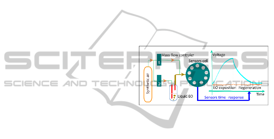
electronic nose. Figure 1 presents the functional

diagram of this experimental system.

The EO generation is made by bubbling

synthetic air flow in a bottle containing 1cm

liquid essential oil. To produce a desired EO diluted

atmosphere at a constant total flow rate, the created

odorant atmosphere is combined with pure air, and

then introduced into the gas sensor cell. So, various

concentrations are obtained by varying the flow rate

of the EO line to be combined with the pure air flow

rate. These EO concentrations (dilutions) are then

expressed as a percentage of the bubbling flow rate

in liquid oil over the total flow rate (100ml/min).

Pine oil at very low percentages (1, 2, 3, and 4%)

is utilized in this study. These concentrations

correspond to a pleasant odour (human panel) for

aromatherapy uses (Sambemana, Siadat and

Lumbreras, 2010). Gas chromatography

measurements were made on the EO pine samples

before the beginning and during the experiment

phase in order to control the stability of the EO

sample composition (molecules and their

concentrations).

The gas sensor cell contains 9 sensors

(TGS2620, TGS880, TGS822, TGS816, SPAQ1,

SPMW0, SP31, MQ3, MQ138) from Figaro, FIS

and Hanwei companies. Sensor responses are

digitalized and collected using a fast and high

resolution data acquisition board. The whole system

will be optimized for an accurate and rapid EO

concentration evaluation. In the functional diagram

(figure 1), we present also a sensor time-response in

terms of sensor voltage response versus time. The

signal shows first a voltage increase with an

inflexion point, corresponding to the gas exposition.

The second part corresponds to the sensor

regeneration.

Figure 1: Functional diagram of the gas sensor

characterization system.

2.2 Feature Determination

After each gas exposition, a sensor regeneration

must be undertaken to recover the conductance basis

value of the sensor. In previous studies, we used a

cycle composed of 5 minutes gas exposition time

followed by 20 minutes regeneration time. This

cycle allowed to obtain sensor response stabilization

during the exposition phase for all the sensors and

all the EO concentrations, and also a good

regeneration at the end of the purge phase.

We have tested many characteristic parameters

corresponding to transient and steady-state phases

(Szczurek and Maciejewska, 2012; Gualdron et al.,

2004), and then selected for this study two features:

one extracted from the sensor time-response, and the

second from the derivative curve of this response.

We have compared the performance of these two

features to discriminate the EO concentrations in

order to choose the best sensors acting with the

shortest measurement cycle, necessary for a real

time application.

2.2.1 Derivative Feature

To have a rapid evaluation of the gas concentration,

SENSORNETS2014-InternationalConferenceonSensorNetworks

238

it is necessary to consider the transient phase of the

sensor time-response (Ionescu, Vancu and Tomescu,

2000; Martinelli et al., 2003; Pardo and Sberveglieri,

2007). More we wait for a complete stabilization,

more the exposition time is long, and longer will be

the regeneration time. In our application, for several

studied cases (towards the sensors and/or the gas

concentrations) the time-response needs more than 5

minutes to reach 90% of the stabilization level.

The most studied transient feature is the initial

slope of the time-response signal (Sysoev et al.,

2007; Delpha, Siadat and Lumbreras, 2001). But the

difficulty is to determine the starting and the end

points of the linear transient phase. It is impossible

to fix a general rule for the calculation of this slope

because these points vary along with the gas

concentration and the sensor types.

So, we have decided to differentiate all the signal

time-responses in order to determine the maximum

of the derivative curve corresponding to the

inflexion point of the sensor time-response. To

reduce noise in the derivative signal, it was needed

the use of an adapted filtering. Several approaches

were tested as Butterworth low pass filtering,

Savitzky-Golay (S-G) derivative and smoothing

filter, and polynomial fitting (Savitzky and Golay,

1967).

(a)

(b)

Figure 2: Raw and filtered time-response signals of a gas

sensor (a) and their respective derivative curves (b) : Peak

apparition in the derivative curve.

The best results were obtained with S-G filter.

For each sensor, filter parameters (window width

and filter order) were adjusted whatever the used

concentration. Figure 2b underlines a notable

maximum of the derivative curve, obtained after

using an adequate filtering. This peak appears

generally in the 75 first seconds, and the height

value depends on the applied gas concentration and

the studied sensor.

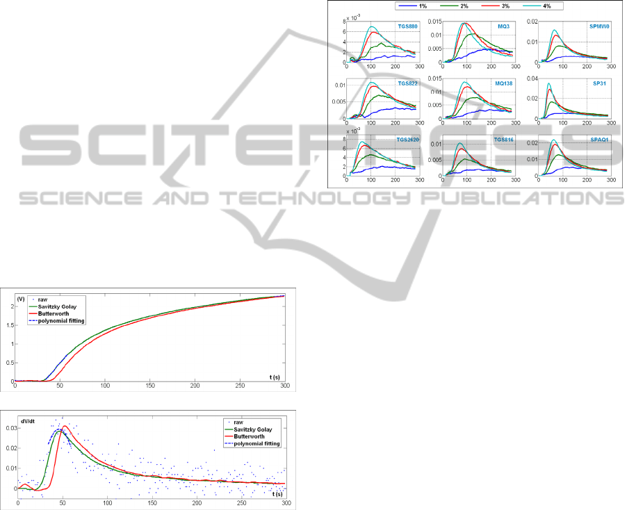
In Figure 3 we present the derivative curves of

the 9 sensors for all the used concentrations. On this

figure the four concentrations are represented using

different colours. For the gas sensors (except MQ3

sensor), the peak height varies clearly with the

concentration. For MQ3 sensor, the superposition of

3% and 4% curves will be explained later.

Figure 3: Derivative curves (dV/dt) of each sensor versus

exposition time (s) along with the four EO concentrations.

2.2.2 Traditional Features

In most of electronic nose applications the

stabilization value of the sensor conductance is used.

To compare the Peak feature with this traditional

feature, we have determined the (Vs-V0) parameter

where Vs is the sensor response value at the end of

the exposure time and V0 the value of the initial

sensor level before the introduction of the EO

vapours.

Vs and V0 values are respectively calculated by

averaging five recorded data at the end and the

beginning of the sensor time-response signal, in

order to reduce the noise effects. The duration of V0

level is short (about 5 to 10 seconds according to the

sensor type) so 5 recorded data are used to average

the V0 value. Concerning Vs, this chosen average

gives satisfactory noise reducing.

In Figure 4 the time responses of all the sensors

for all the concentrations are drawn. We note that we

only obtain a good separation along with the

concentration for a few sensors (TGS2620, TGS880,

TGS816). The other sensors show high sensitivity to

the EO atmospheres than the three first cited sensors

with early sensor saturation. So, we see on the

corresponding graphs that the saturation occurs from

3% and even from 2% for the MQ3 sensor.

SensorsandFeaturesSelectionforRobustGasConcentrationEvaluation

239

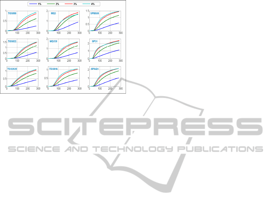
Figure 4: Response signals (V) of each sensor versus

exposition time (s) along with the four EO concentrations.

2.2.3 Discussion

The choice of the sensors is predominant for a

reliable discrimination with electronic nose systems.

We have seen (Figure 4) that the saturation of the

sensor time-response occurs unfortunately for many

sensors, because of their high sensitivity to the

concerned effluent. So, for these sensors the

traditional parameter (Vs-V0) cannot well indicate

the concentration variation.

Concerning the “transient” parameter, Peak,

deduced from the derivative curve, the results

(Figure 3) show a better efficiency to discriminate

the concentration. In fact, this value is obtained

during the transient phase of the sensor time-

response (<75 seconds), then it is less influenced by

the saturation (excepted for MQ3 sensor).

So, these observations lead us to optimize our

detection system by reducing as much as possible

the gas exposition time. Consequently this reduction

might implicate the regeneration time reduction,

taking into account that these two phase times are

not linearly related.

This optimization is advantageous in two ways:

to reduce the measurement time and to improve the

efficiency of the traditional (Vs-V0) feature. This

approach will allow us to select the best sensors for

our real-time application.

3 MEASUREMENT

OPTIMIZATION

In this section we develop the optimization of the

measurement protocol, particularly important for

real time applications. After discussion about the

choice of the gas exposure and purge times, we

insist on the disparity between the sensor

behaviours. The study of these disparities permits us

to select the best sensors according to the optimized

measurement procedure and application.

3.1 Protocol Optimization

We know that measurement cycle has to be

composed of the gas exposure phase followed by the

sensor regeneration phase. In the considered

application, we need to determine the EO

concentration as quickly as possible, so one of our

goal was to reduce the times corresponding to the

measurement and regeneration phases with respect

of a good sensor regeneration.

So, several Exposure-Regeneration times were

tested. These experiments show us first that, even if

the exposure time becomes extremely short (for

example 60 seconds), the regeneration time remains

still very long (about 300s) to obtain a satisfactory

sensor layer cleaning. We have also noted that these

times are strongly related to the sensor type and of

course, for each sensor they depend on the used gas

concentration.

For each value of the studied exposition time,

several values of the regeneration time were applied

to control the sensor recovery. For an exposition

time less than 75s, the sensor time response does not

reach either the stabilization value, either the

inflexion point. So, it is impossible to determine a

reliable value of Peak (maximum of the derivative

curve). In contrary, an exposition time of 75 seconds

is convenient for all the sensors and most of the pine

EO concentrations. We have tested several

regeneration times for this exposition time. Figure 5

presents a set of cycles in the cases (a: 75s-150s) and

(b: 75s- 350s). In the case (a), all the graphs show an

important drift of the sensor initial values. The

sensor regenerations are not sufficient. In the case

(b), the regeneration is practically obtained for most

of the sensors. Other protocol (100s-500s) has given

practically the same results than the protocol (75s-

350s). This last cycle protocol is adopted for our

next investigation. This choice takes into account the

importance of a rapid and accurate measurement.

3.2 Sensor Selection

After adopting the measurement protocol, we looked

into the matter of the gas sensor selection. As we can

see on the Figure 5b, several sensors (TGS816,

TGS2620, SPAQ1, SPMW0 sensors) show a good

recovery into their initial conductance value after the

SENSORNETS2014-InternationalConferenceonSensorNetworks

240

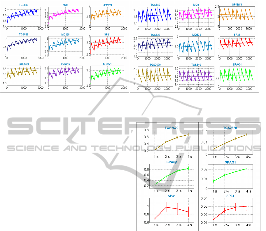
(a) (b)

Figure 5: Set of repetitive Exposure-Regeneration cycles for all the sensors and 2% pine oil in the case of (a): 75s-150s and

(b) 75s-350s exposure and regeneration times.

regeneration phase. The other sensors present weak

or important drift, generally because they give a high

response to the EO atmospheres.

As we had characterized nine sensors, we

compared the recovery process of each sensor for all

the used EO concentrations. For this comparison we

have determined the Peak and the (Vs-V0) features.

The mean value and the corresponding standard

deviation are calculated from all the measurements

(8 repetitions), for each sensor and each EO

concentration. These values are plotted on the

Figure 6 for three representative sensors. We note

that the TGS2620 is the more appropriate for pine

EO concentrations discrimination: the values of

Peak and (Vs-V0) features show a very sensible rise

along the EO concentration with weak standard

deviations. But we can surprisingly see the

inefficiency of the SP31 sensor for this application.

Because of its high sensitivity to pine atmosphere,

the saturation occurs after 1% EO, represented by

abnormal evolution of the (Vs-V0) and Peak values

versus EO concentration. For the SPAQ1 sensor the

behaviour is intermediate, with a good variation of

Peak and a rather less efficient variation of (Vs-V0),

essentially higher than 3% EO concentration.

This comparison study leads us to detect three

qualities of sensors among our sensor array: very

good, good and non-adapted sensors for the

concerned protocol and application.

 Very good: TGS 2620, TGS 880, SPMW0

 Good: TGS 816, TGS822, SPAQ1, MQ138

 Non-adapted: SP31, MQ3

(a) (b)

Figure 6: Feature evolutions of 3 gas sensors versus pine

EO concentrations (1, 2, 3, 4%); (a) Vs-V0, (b) Peak.

3.3 PCA Results

The measurements made for all the concentration

range (1, 2, 3, 4%) were analysed by Principal

Component Analysis (PCA) using as explicative

variables one of the two selected features (Peak or

(Vs-V0) of the nine sensors) separately. So, nine

principal components are obtained by linear

combinations of the original variables and

participate decreasingly to the construction of the

model. Figure 7 shows on the first two principal

components (PC1 and PC2) the loadings plots of

each of the two variable sets. A loading plot present

the correlation between the concerned variables, so

SensorsandFeaturesSelectionforRobustGasConcentrationEvaluation

241

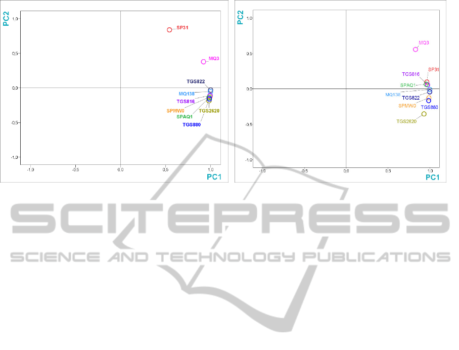
(a) (b)

Figure 7: PCA loading plots; (a) Vs-V0 with PC1 explaining 88.9% of the variation and PC2 10.6%; (b) Peak with PC1

explaining 91.6% of the variation and PC2 5.5%.

all the representative points are positioned inside a

unit length circle, called “circle of correlation”.

In our case, each variable characterises one of

the nine gas sensors. So, the loading plot, given by

PCA, provides a map of how the sensors relate to

each other. In this map, the more sensor projections

are closed together, the more they present similar

properties. Furthermore, the distance to the origin of

PC1 and PC2 also conveys information: the further

away from the plot origin a variable is located, the

stronger impact that variable has on the model with

respect of the EO concentration separation. The

more a variable is close to the origin of the plane,

the less important it is (Berna, Anderson and

Trowell, 2009; Jolliffe, 2002). In the same way,

since the PC1 explains the most important part of the

variation than PC2, this impact is stronger when the

variable is near to the unit length of PC1.

In Figure 7(a), where (Vs-V0) feature of each

sensor is used as representative variable, we can note

that SP31 and MQ3 sensors are situated far from the

unit length of the PC1. They are then less adapted

than the other sensors. This observation confirms the

previous result about the efficiency of these two

sensors. Other sensors of the array are positively

correlated and satisfy the condition of strong impact.

Considering Figure 7(b) where Peak is used as

representative feature, we can observe that the SP31

sensor becomes more efficient and joints other group

of sensor with high impact. But MQ3 sensor is

definitively less adapted for this study.

These PCA results confirm our sensor behaviour

study (section 3.2).

4 CONCLUSIONS

We have shown through this work that a deep

evaluation of the sensor behaviour according to the

studied atmosphere is required for reliable electronic

nose application such as gas quantification. Two

features extracted from the transient and the steady-

state phases of the sensor response signal (Peak: the

maximum of the derivative signal of sensor

response, and (Vs-V0): the response amplitude

voltage) were studied and compared. The

performance of the unusual Peak feature is

highlighted to provide fast and continuous

measurement. The capacity of this feature to

quantify pine oil vapour diffused in pure air has

permitted the optimization of the measurement time

conditions and also the selection of the best sensors.

In fact we have shown important disparities on the

stability and the performance of the chosen features

along with the sensor types. Loading plots obtained

with PCA confirm these results.

REFERENCES

Berna, A. Z., Anderson A. R., Trowell S. C., 2009. Bio-

Benchmarking of Electronic Nose Sensors. PLoS

ONE, 4(7): e6406;

[Online]; doi: 10.1371/journal.pone.0006406.

Boilot, P., Hines, E. L., Gongora, M. A., Folland, R. S.,

2002. Electronic noses inter-comparison, data fusion

and sensor selection in discrimination of standard fruit

solutions. In Sensors and Actuators B, 88, 80-88.

SENSORNETS2014-InternationalConferenceonSensorNetworks

242

Branca, A., Simonian, P., Ferrante, M., Novas, E., Martin

Negri R., 2003. Electronic based discrimination of a

perfumery compound in a fragrance. In Sensors and

Actuators B, 92, 222-227.

Cho, J. H., Kim, Y. W., Na, K. J., Jeon G. J., 2008.

Wireless electronic nose system for real-time

quantitative analysis of gas mixtures using micro-gas

sensor array and neuro-fuzzy network. In Sensors and

Actuators B, 134, 104-111.

Delpha, C., Siadat, M., Lumbreras, M., 2001. An

electronic nose using time reduced modelling

parameters for a reliable discrimination of Forane

134a. In Sensors and Actuators B, 77, 517-524.

Distante, C., Leo, M., Siciliano, P., Persaud, K.C., 2002.

On the study of feature extraction methods for an

electronic nose. In Sensors and Actuators B, 87, 274-

288.

Falasconi, M., Pardo,M., Sberveglieri, G., Ricco, I.,

Bresciani, A., 2005. The novel EOS

835

electronic nose

and data analysis for evaluating coffee ripening. In

Sensors and Actuators B, 110, 73-80.

Gualdron O., Llobet E., Brezmes J., Vilanova X., Correig,

X., 2004. Fast variable selection for gas sensing

applications. In Sensors, 2004. Proceeding of IEEE, 2,

892-895.

Gutierrez-Osuna R., 2002. Pattern analysis for machine

olfaction: A review. In IEEE Sensor Journal, 2, 189-

202.

Ionescu, R., Vancu, A., Tomescu, A., 2000. Time-

dependent humidity calibration for drift corrections in

electronic noses equipped with SnO2 gas sensors. In

Sensors and Actuators B, 69, 283-286.

Jolliffe, I.T., 2002. Principal Component Analysis, Second

edition. New York: Springer.

Llobet, E., Ionescu, R., Al-Khalifa, S., Brezmes, J.,

Vilanova, X., Correig, X., Barsan, N., Gardner, J.W.,

2002. Multicomponent gas mixture analysis using a

single tin oxide sensor and dynamic pattern

recognition. In Sensors Journal, IEEE, 1 (3), 207-213.

Martin Negri R. and Reich S., 2001. Identification of

pollutant gases and its concentrations with a

multisensory array. In Sensors and Actuators B, 75,

172-178.

Martinelli, E., Falconia, C., D’Amico A., Di Natale, C.,

2003. Feature Extraction of chemical sensors in phase

space. In Sensors and Actuators B, 95, 132–139.

Pardo, M. and Sberveglieri. G., 2007. Comparing the

performance of different features in sensor arrays. In

Sensors and Actuators B, 123, 437–443.

Paulsson, N., Larsson, E., Winquist, F., 2000. Extraction

and selection of parameters for evaluation of breath

alcohol measurement with an electronic nose. In

Sensors and Actuators B, 84, 187-197.

Roussel, S., Forberg, G., Grenier P., Bellon-Maurel, V.,

1999. Optimisation of electronic nose measurements.

partII : Influence of experimental parameters. In

Journal of Food Engineering, 39, 9-15.

Sambemana, H., Siadat, M., Lumbreras, M., 2010. Gas

sensing evaluation for the quantification of natural oil

diffusion. In Chemical Engineering Transaction, 23,

177-183.

Savitzky, A. and Golay, M.J.E., 1967. Smoothing and

Differentiation of Data by Simplified Least

SquaresProcedures. In Anal. Chem., 36 (8), 1627–

1639.

Sysoev, V. V., Goschnick, J., Schneider, T., Strelcov, E.,

Kolmakov, A., 2007. A gradient microarray electronic

based on percolating SnO2 nanowire sensing

elements. In Nano letters, 7 (10), 3182-3188.

Szczurek, A. and Maciejewska, A., 2012. Gas Sensor

Array with Broad Applicability, Sensor Array, Prof.

Wuqiang Yang (Ed.), ISBN: 978-953-51-0613-5,

InTech. Available from: http://www.intechopen.com/

books/sensor-array/gas-sensor-array-with-broad-

applicability.

Zhang, S., Xie, C., Zeng, D., Zhang, Q., Li, H., Bi, Z.,

2007. A feature extraction method and a sampling

system for fast recognition of flammable liquids with a

portable E-nose. In Sensors and Actuators B, 124,

437-443.

Zhang, H. and Wang, J., 2007. Detection of age and insect

damage incurred by wheat, with an electronic nose. In

Journal of Stored Products Research, 43, 489-495.

SensorsandFeaturesSelectionforRobustGasConcentrationEvaluation

243