
Detecting Unusual Inactivity by Introducing Activity Histogram
Comparisons
Rainer Planinc and Martin Kampel
Computer Vision Lab, Vienna University of Technology, Favoritenstrasse 9-11/183-2, A-1040 Vienna, Austria
Keywords:
Inactivity Detection, Activity Modeling, Ambient Assisted Living, Histogram
Abstract:
Unusual inactivity at elderly’s homes is an evidence that help is needed. Hence, the automatic detection of
abnormal behaviour with a low number of false positives is desired. The aim of this work is to improve the
accuracy of inactivity detection by introducing a new approach based on histogram comparison in order to
reliably detect abnormal behaviour in elderly’s homes. The proposed approach compares activity histograms
with a pre-trained reference histogram and detects deviations from normal behavior. Evaluation is performed
on a dataset containing 103 days of activity, where six days were reported as containing ”unusual” inactivity
(i.e., longer absence from home) by an elderly couple.
1 INTRODUCTION
Ambient Assisted Living (AAL) solutions are devel-
oped to assist elderly and enable them to stay in their
own homes longer. Due to the demographic change
in Europe, assistive technologies are needed to ful-
fill the raising demand of taking care. A focus in the
development of AAL technologies is to detect criti-
cal events and provide help as soon as possible since
this reduces the mortality rate (Noury et al., 2008).
Fall detection focuses on the critical event of falling
down and being not able to get up on your own and
approaches to detect falls are proposed (e.g., (Lee
and Chung, 2012; Anderson et al., 2006; Nait-Charif
and McKenna, 2004; Planinc and Kampel, 2012)).
These approaches use computer vision to detect falls
in home environments and thus provide unobtrusive
AAL solutions. However, not only falls are critical
events to be detected, but also changes in the daily
routine of the elderly indicate situations where help
is needed (e.g., due to illness). Human action recog-
nition (Ballin et al., 2013) can be used to detect and
model actions which are performed during the daily
routine, but focus on the pre-defined actions.
Since the type of actions elderly perform dur-
ing the day is not relevant for the detection of un-
usual inactivity, the authors of this work focus on a
more generic approach. Similar work is performed
by Floeck & Litz (Floeck and Litz, 2008) and Cud-
dihy et al. (Cuddihy et al., 2007). They introduced
an approach to model inactivity and to detect unusual
inactivity by only considering motion data, indepen-
dently from the source of data (e.g., motion data is
obtained by motion sensors, door sensors).
The aim of this paper is the introduction of a
histogram based activity modeling approach and the
detection of unusual (in)activity while reducing the
number of false alarms. Activity data is obtained by
using tracking information from the OpenNI tracker
NITE and an Asus Xtion pro, but can be obtained by
any arbitrarily tracking algorithm or sensor type (e.g.,
motion sensor). Tracking information consists of the
center of mass of a person and the timestamp when
motion (activity) is detected. If more than one person
is present, only tracking information of one person is
stored, since this indicates activity and the number of
people being present is not relevant for this approach.
The rest of this paper is structured as follows:
Section 2 presents the state of the art in the field of
unusual inactivity detection whereas Section 3 intro-
duces the proposed approach. An evaluation in Sec-
tion 4 demonstrates the feasibility of our approach
and finally a conclusion is drawn in Section 5.
2 STATE-OF-THE-ART
Nait-Charif & McKenna (Nait-Charif and McKenna,
2004) use tracking information from an overhead
camera to summarize activity in home environments.
The movement of the person is tracked and the room
313
Planinc R. and Kampel M..
Detecting Unusual Inactivity by Introducing Activity Histogram Comparisons.
DOI: 10.5220/0004670203130320
In Proceedings of the 9th International Conference on Computer Vision Theory and Applications (VISAPP-2014), pages 313-320
ISBN: 978-989-758-004-8
Copyright
c
2014 SCITEPRESS (Science and Technology Publications, Lda.)
is divided into entry/exit zones, inactivity zones and
transition areas. A typical use of the room is modeled
as follows: a person enters the room via an entry zone,
moves to one or more inactivity zones and finally
leaves the room via an exit zone. Transition areas are
defined to be areas where the transition from an en-
try/exit zone to an inactivity zone or between inactiv-
ity zones take place. Inactivity zones are learned auto-
matically using the approach introduced in (McKenna
and Nait-Charif, 2004). The person’s speed is ana-
lyzed to define whether the person is active or inac-
tive. Depending on the location of the person during
the inactivity, the system detects whether the inactiv-
ity occurs in an already pre-defined inactivity area or
outside such areas. This allows to detect unusual in-
activity which can be caused by a fall. Furthermore,
activity patterns (i.e., sequence of visiting different
zones) are analyzed and deviations of patterns are de-
tected. However, the work of Nait-Charif & McKenna
(Nait-Charif and McKenna, 2004) focus on spatial as-
pects of inactivity, but temporal aspects are not taken
into consideration since only the sequence of visiting
zones is analyzed but not associated with the time of
the day (e.g., the sequence of visiting different zones
may change depending on the time).
In contrast, Floeck & Litz (Floeck and Litz, 2008)
and Cuddihy et al. (Cuddihy et al., 2007) focus on
temporal aspects of inactivity. Activity data is col-
lected using 30 sensors (i.e., motion detectors, door
and window sensors) resulting in an activity profile
(Floeck and Litz, 2008). However, due to the diver-
sity of sensors used, inactivity profiles are introduced
to combine the data from different sensors to one pro-
file. An inactivity profile is constructed by analyzing
the duration of inactivity over time, where inactivity
is defined as no activity from any sensor. As long as
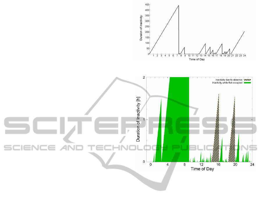
no activity is detected, the duration of inactivity raises
over time, shown in Figure 1. If any kind of activity
is detected, the inactivity duration is set to zero (e.g.,
between 7 and 8 AM). Afterwards, the inactivity dura-
tion raises since no activity is detected between 8 and
9 AM. Due to the combination of motion and door
sensors, the approach proposed in (Floeck and Litz,
2008) is able to differentiate between inactivity due to
absence of the person (data obtained by door sensors)
and inactivity when the person is present. Figure 2 de-
picts an inactivity diagram, distinguishing whether a
person is present or absent when inactivity is detected.
In order to detect abnormal inactivity, the inac-
tivity profile is compared to a pre-trained reference
profile (e.g., average inactivity profile of one month).
Therefore, the profiles are divided into n different
time slots. Floeck & Litz (Floeck and Litz, 2008) cal-
culate the integral of inactivity of each time slot and
Figure 1: Inactivity profile.
Figure 2: Inactivity profile considering data different sensor
types (Floeck and Litz, 2008).
combine all n time slots to one feature vector per day,
which is compared to the reference vector using the
Dice coefficient (Dice, 1945). By introducing a tol-
erance value and a convolution with a weighting vec-
tor, small temporal and numerical deviations are com-
pensated (e.g., sleeping 5 minutes longer than usual).
Since the inactivity profiles are compared on a one-
day vector basis, deviations are detected at the end
of the day. However, extensive evaluation of this ap-
proach is missing and thus no performance measures
when being applied to real world scenarios can be ob-
tained.
Cuddihy et al. (Cuddihy et al., 2007) use door
sensors to detect if a person leaves the flat in order to
minimize false positives when no person is present.
Similar to (Floeck and Litz, 2008), the authors use in-
activity profiles and each day is divided into n time
slots. A reference alert line is learned over the dura-
tion of 45 days by analyzing the maximal inactivity
duration at each time slot and adding buffers to allow
small deviations. The uniform and variable buffer act
as vertical tolerance and ensure, that the sensitivity of
the algorithm is adopted according to the amount of
inactivity (i.e., the algorithm is more sensitive during
active times and less sensitive during inactive times).
Furthermore, time shifts are compensated by apply-
VISAPP2014-InternationalConferenceonComputerVisionTheoryandApplications
314

ing a weighting function to the inactivity data and
thus considering also adjacent intervals providing a
temporal buffer. Each time interval is compared to
the corresponding time interval of the alert line im-
mediately, hence alarms are raised at the end of each
time interval. The alert line is adopted based an a 45
days rolling window approach, hence the alert line is
learned from the last 45 days and adopts to behavioral
changes automatically.
3 METHODOLOGY
Floeck & Litz (Floeck and Litz, 2008) and Cuddihy
et al. (Cuddihy et al., 2007) use inactivity profiles
since they argue that it is difficult to combine dif-
ferent signals (start/stop signals and discrete events)
to one common profile. This work focus on dis-
crete events (i.e., motion detected / no motion de-
tected), hence no inactivity profiles need to be cal-
culated to fuse the sensor data. Instead, activity his-
tograms are used to detect unusual inactivity. Since
histogram comparison is widely used in the area of
image processing (e.g., image retrieval), activity his-
tograms are introduced in this work in order to detect
unusual inactivity. Activity data is aggregated in his-
tograms of 24 bins representing one day, resulting in
one bin per hour. The number of bins was choosen
to achieve a trade-off regarding the granularity of the
approach, i.e. the activity is not analyzed in detail
(e.g., per minute) and not per day, but on an hourly
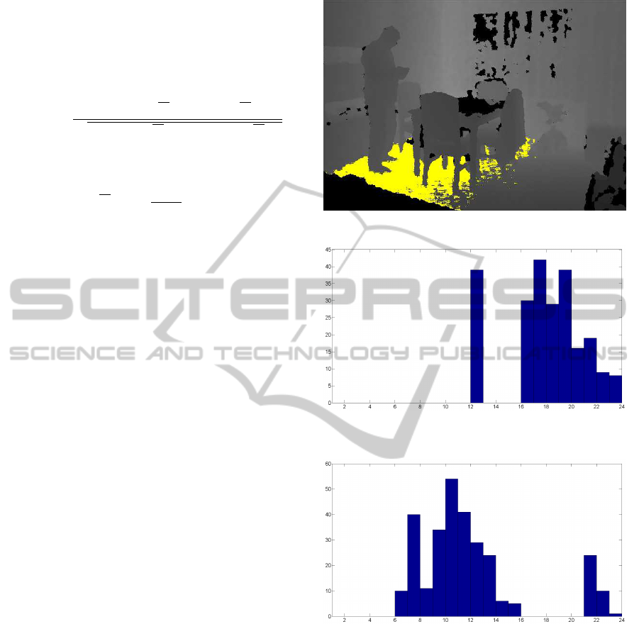
basis. Figure 3 depicts an example of an activity his-
togram (top) and the corresponding inactivity profile
(bottom). Since motion (activity) was detected dur-
ing the night between one and two AM, the inactiv-
Figure 3: Example of an activity and corresponding inactiv-
ity profile.
ity dropped to zero. The inactivity between 8:30 and
9:30 AM is better reflected in the inactivity profile,
since only a smaller amount of activity is depicted in
the activity histogram. But since a temporal buffer
need to be added to detect abnormal inactivity, both
representations are feasible.
During the training phase, the histograms H
n
for
all n training days are calculated. The average his-
togram H
re f
of all histograms H
n
is calculated and
used as a reference for ”normal” behavior. In order
to model the variability of the training data, the dis-
tances d
n
between the nth histogram and the reference
H
re f
are calculated.
The distance matrix D
n
represents the distances
between all bins and the distance d
n
is the sum of all
distances D
i j
, shown in Equation 1.
d
n
=
24
∑
i, j=1
D
i j
(1)
The average distance d and standard deviation σ
are calculated from the training set and used as deci-
sion criteria during the test phase. A deviation from a
normal daily routine is detected if
|d
t
| ≥ d + σ (2)
where d
t
denotes the histogram distance of the day
to be analyzed to the reference histogram H
re f
.
For the calculation of the distances, the euclidean,
chi-square (Cha, 2008), earth mover’s distance (Rub-
ner et al., 2000), bhattacharyya distance (Comaniciu
et al., 2000; Bhattacharyya, 1943) as well as inter-
section (Swain and Ballard, 1991) and the Pearson
Product-Moment Correlation Coefficient (Rodgers
and Nicewander, 1988) are analyzed during the eval-
uation.
The chi-square distance is defined as
d(H
1
, H
2
) =
1
2
∑
i
(H
1
(i) − H
2
(i))
2
H
1
(i) + H
2
(i)
(3)
The earth mover’s distance is calculated by com-
puting the optimal flow f
i j
and the ground distance d
i j
and is defined as
d(H
1
, H
2
) =
∑
i
∑
j
d
i j
f
i j
∑
i
∑
j
f
i j
(4)
The bhattacharyya distance for histograms is
based on the bhattacharyya coefficient and is defined
as
d(H
1
, H
2
) =
v
u
u
t
1 −
∑
i
p
H
1
(i) · H
2
(i)
q
∑
j
H
1
( j) ·
∑
j
H
2
( j)
(5)
DetectingUnusualInactivitybyIntroducingActivityHistogramComparisons
315
The intersection of histograms is defined as
d(H
1
, H
2
) = 1 −
∑
i
min(H
1
(i), H
2
(i)) (6)
The Pearson Product-Moment Correlation Coeffi-
cient is defined as
d(H
1
, H
2
) =
∑
i
(H
1
(i) − H
1
) · (H
2
(i) − H
2
)
p
∑
i
(H
1
(i) − H
1
)
2
·
∑
i
(H
2
(i) − H
2
)
2
(7)
where
H
k
=
∑
i
H
k
(i)
n
(8)
In order to provide a lateral buffer, the histograms
are compared on a daily basis resulting in a delay of
an alarm in comparison to the approach introduced by
Floeck & Litz (Floeck and Litz, 2008), but reducing
the number of false positives dramatically.
4 EVALUATION
The evaluation is based on activity data obtained by
the observation of the living room of an elderly cou-
ple over the duration of 103 days. The monitored field
of view is shown in Figure 4 and covers the area of the
living room, where a table is used for food intake. Six
of the monitored days were reported as ”unusual” by
the couple, i.e., consist longer absence from home or
dramatically changed daily routines. Hence, 97 days
are considered as normal days where no alarm should
be raised. Since this dataset is not artificially altered
but acquired from a real scenario, it might be unbal-
anced with respect to the ratio of alarms and days not
containing an alarm.
Nevertheless, the recorded dataset is challenging,
since it represents the daily activities of real persons,
not considering the change of daily activities during
the week or on the weekend. Only the six days re-
ported by the elderly where marked as alarms and thus
being absent for half a day (Figure 5) is not reported
as ”unusual”, since this is not unusual for the couple.
However, a typical histogram of activities is depicted
in Figure 6: getting up in the morning between 6 and
7 AM followed by a peak of activities due to prepar-
ing and eating breakfast. Moreover, around noon, ac-
tivity is increased due to typical activities performed
during the morning and early afternoon (e.g., eating,
playing cards, reading the newspaper). In the after-
noon, no activity is detected due to watching TV in
another part of the living room followed by activity
due to preparing and eating dinner. Figure 7 depicts
a similar histogram of activity, although the shape is
Figure 4: Part of the living room being monitored.
Figure 5: Example of a normal day 1 - activity in the morn-
ing is missing, but this day is considered as normal activity.
Figure 6: Example of a normal day 2 - activity is present
throughout the day, except the afternoon.
different compared to Figure 6 due to a changed inten-
sity of performing activities. Figure 8 shows an ”un-
usual” behavior due to enhanced activity in the morn-
ing but decreased activity during the day (the amount
of activity is significantly lower than ”normal”). An
abnormal shape of activity is depicted in Figure 9 and
thus results in being categorized as ”unusual” activ-
ity. Absence for almost the whole day is also reported
as ”unusual” since usually at least one person of the
elderly couple is at home during the day (e.g., around
noon), depicted in Figure 10.
Evaluation results are obtained by varying the
number n of randomly choosen training days from
VISAPP2014-InternationalConferenceonComputerVisionTheoryandApplications
316
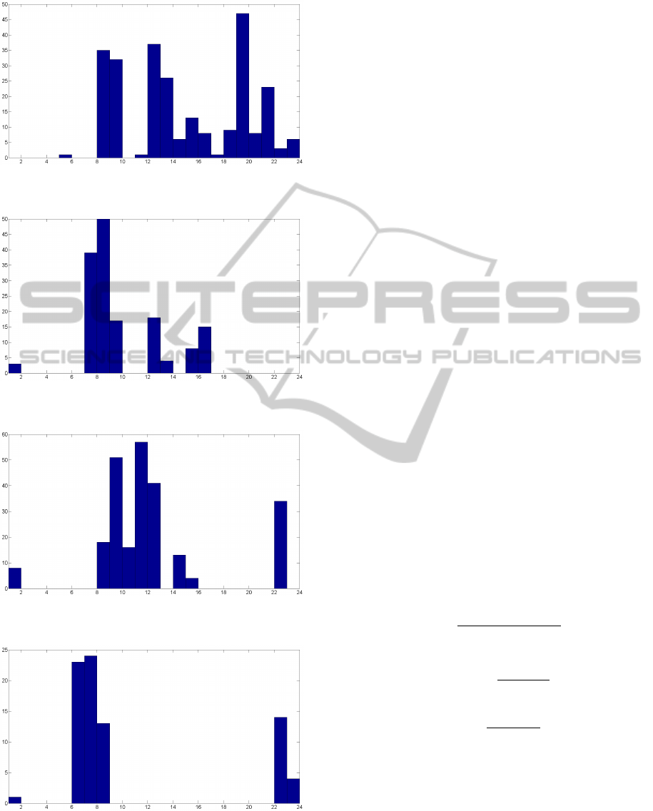
Figure 7: Example of a normal day 3 - activity and inactivity
are present throughout the day.
Figure 8: Example of unusual activity 1 - activity is reduced
in the afternoon/evening.
Figure 9: Example of unusual activity 2 - no activity in the
afternoon/evening.
Figure 10: Example of unusual activity 3 - absence during
the day.
two up to 97 training days. The six days reported
as abnormal behavior were not included in the train-
ingset, but in the testset. Thus, the size of the testset
is 101 to six test samples, depending on the training
set.
Since inactivity detection often results in false
alarms, the goal is to reduce the number of false pos-
itives while detecting true positives. The proposed
approach is evaluated using the toolbox provided by
(Doll
´
ar, 2012) and compared to the approach using an
alert line introduced by Cuddihy et al. (Cuddihy et al.,
2007). Evaluation results, depicted in Figure 11, visu-
alize the number of alarms depending on the number
of training days. As can be clearly seen, the num-
ber of false alarms using the alert line approach is
high, especially with only few trainingdata (over 500
alarms when using 2 days of training data). In com-
parison, using the proposed approach, the number of
false alarms when using few training data is reduced
to less than 100 false alarms. Please note that 100
resp. 500 false alarms on a testset including 101 test
days results in one resp. five false alarms per day
in average. Figure 12 shows a detailed view of Fig-
ure 11, where the maximum number of alarms is cut
off at 100 in order to enhance the comparability be-
tween the approaches.
In order to improve the accuracy of the system,
more training data is needed . However, even when in-
creasing the trainingset to the size of 45 days, which is
proposed by Cuddihy et al. (Cuddihy et al., 2007), the
proposed approach still reduces the number of alarms
from 35 when using the alert line approach to less
than 16 alarms using the proposed approach. Since
six alarms are included in the testset, the number of
false positives is even lower.
In order to evaluate the accuracy of the system, the
f-score (C. J. van Rijsbergen, 1979) is calculated and
plotted depending on the size of the trainingset. The
f-score is defined as
F = 2 ·
precision · recall
precision + recall
(9)
with
precision =
T P
T P + FP
(10)
and
recall =
T P
T P + FN
(11)
where TP is the number of true positives, FP the
number of false positives and FN the number of false
negatives. Figure 13 depicts the f-scores of the intro-
duced approach using different distance measures and
the f-score of the alert line approach. All distances
except the earth mover’s distance and the correla-
tion clearly outperform the alert line method (Cud-
dihy et al., 2007), not only in terms of less alarms but
also in terms of better f-score values. The histogram
DetectingUnusualInactivitybyIntroducingActivityHistogramComparisons
317
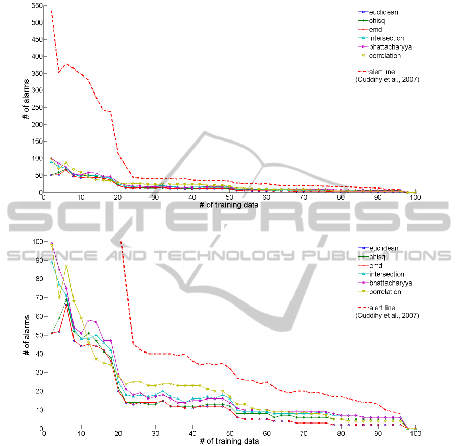
Figure 11: Alarm rate depending on the size of the training sample.
Figure 12: Detailed view of alarm rate (number of alarms ≤ 100) depending on the size of the training sample.
correlation performs similar to the alert line approach,
whereas the earth mover’s distance results in a lower
f-score than the alert line approach.
Table 1 depicts the number of alarms depending
on the size of the training data. All histogram com-
parisons perform better in comparison to the alert line
approach in terms of less false positives. However, the
number of alarms do not indicate whether the alarm
is a true or false positive and thus the f-score is cal-
culated and used for comparison of these approaches,
e.g., the number of alarms using the euclidean dis-
tance and the earth mover’s distance result in the same
number of alarms, but in different f-scores due to con-
sideration of true and false positives when calculating
the f-score.
Table 2 illustrates the accuracy of the proposed
approach using different distance measures and com-
pares the results to the alert line method introduced
in (Cuddihy et al., 2007). The highest f-score values
are marked bold and thus can be seen that the chi-
square distance performs best and increases the accu-
racy compared to the alert line approach.
5 CONCLUSIONS
This work introduced the comparison of activity his-
VISAPP2014-InternationalConferenceonComputerVisionTheoryandApplications
318
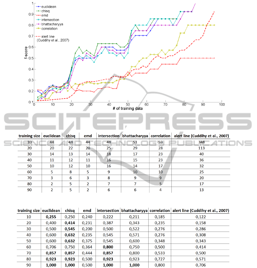
Figure 13: f-score depending on the size of the training sample.
Table 1: Number of alarms.
Table 2: F-score.
tograms to detect unusual inactivity. In contrast to
state-of-the-art methods, activity histograms are used
without constructing inactivity profiles. A reference
activity histogram is learned over time and the deci-
sion if an abnormal long inactivity occurred is based
on histogram comparison. This approach was evalu-
ated on a dataset containing 103 days of tracking data
obtained from an elderly couple and results showed,
that the proposed approach outperforms the alert line
approach, when using appropriate distance measures
(e.g., the chi-square distance).
ACKNOWLEDGEMENTS
This work is supported by the European Union under
grant AAL 2010-3-020.
REFERENCES
Anderson, D., Keller, J. M., Skubic, M., Chen, X., and He,
Z. (2006). Recognizing falls from silhouettes. In 28th
Annual International Conference of the IEEE on En-
DetectingUnusualInactivitybyIntroducingActivityHistogramComparisons
319

gineering in Medicine and Biology Society, 2006., vol-
ume 1, pages 6388–6391, New York.
Ballin, G., Munaro, M., and Menegatti, E. (2013). Human
Action Recognition from RGB-D Frames Based on
Real-Time 3D Optical Flow Estimation. In Chella,
A., Pirrone, R., Sorbello, R., and J
´
ohannsd
´
ottir, K. R.,
editors, Biologically Inspired Cognitive Architectures
2012, volume 196 of Advances in Intelligent Systems
and Computing, pages 65–74. Springer Berlin Heidel-
berg.
Bhattacharyya, A. (1943). On a measure of divergence
between two statistical populations defined by their
probability distributions. Bull. Calcutta Math. Soc,
35(99-109):4.
C. J. van Rijsbergen (1979). Information Retrieval. Butter-
worth.
Cha, S.-H. (2008). Taxonomy of nominal type histogram
distance measures. In Proceedings of the Ameri-
can Conference on Applied Mathematics, MATH’08,
pages 325–330, Stevens Point, Wisconsin, USA.
World Scientific and Engineering Academy and So-
ciety (WSEAS).
Comaniciu, D., Ramesh, V., and Meer, P. (2000). Real-
time tracking of non-rigid objects using mean shift.
In Computer Vision and Pattern Recognition, 2000.
Proceedings. IEEE Conference on, volume 2, pages
142–149 vol.2.
Cuddihy, P., Weisenberg, J., Graichen, C., and Ganesh, M.
(2007). Algorithm to automatically detect abnormally
long periods of inactivity in a home. In Proceed-
ings of the 1st ACM SIGMOBILE international work-
shop on Systems and networking support for health-
care and assisted living environments, HealthNet ’07,
pages 89–94, New York, NY, USA. ACM.
Dice, L. R. (1945). Measures of the Amount of Ecologic
Association Between Species. Ecology, 26(3):297–
302.
Doll
´
ar, P. (2012). Piotr’s Image and Video Matlab Toolbox
(PMT). http://vision.ucsd.edu/%7Epdollar/toolbox/
doc/index.html. [Online; accessed 07-November-
2013].
Floeck, M. and Litz, L. (2008). Activity- and Inactivity-
Based Approaches to Analyze an Assisted Living En-
vironment. In Second International Conference on
Emerging Security Information, Systems and Tech-
nologies, 2008. SECURWARE ’08., pages 311–316.
Lee, Y.-S. and Chung, W.-Y. (2012). Visual sensor based
abnormal event detection with moving shadow re-
moval in home healthcare applications. Sensors
(Basel, Switzerland), 12(1):573–84.
McKenna, S. J. and Nait-Charif, H. (2004). Learning spa-
tial context from tracking using penalised likelihoods.
In Proceedings of the 17th International Conference
on Pattern Recognition (ICPR), volume 4, pages 138–
141 Vol.4.
Nait-Charif, H. and McKenna, S. (2004). Activity summari-
sation and fall detection in a supportive home environ-
ment. In Proceedings of the 17th International Con-
ference on Pattern Recognition (ICPR), pages 323–
326 Vol.4. IEEE.
Noury, N., Rumeau, P., Bourke, A. K., OLaighin, G., and
Lundy, J. E. (2008). A proposal for the classification
and evaluation of fall detectors. Biomedical Engineer-
ing and Research IRBM, 29(6):340–349.
Planinc, R. and Kampel, M. (2012). Robust Fall Detection
by Combining 3D Data and Fuzzy Logic. In Park, J.-I.
and Kim, J., editors, ACCV Workshop on Color Depth
Fusion in Computer Vision, pages 121–132, Daejeon,
Korea. Springer.
Rodgers, J. L. and Nicewander, W. A. (1988). Thirteen
Ways to Look at the Correlation Coefficient. The
American Statistician, 42(1):59–66.
Rubner, Y., Tomasi, C., and Guibas, L. (2000). The Earth
Mover’s Distance as a Metric for Image Retrieval.
International Journal of Computer Vision, 40(2):99–
121.
Swain, M. and Ballard, D. (1991). Color indexing. Interna-
tional Journal of Computer Vision, 7(1):11–32.
VISAPP2014-InternationalConferenceonComputerVisionTheoryandApplications
320
