
RAID’ing Wireless Sensor Networks
Data Recovery for Node Failures
Ailin Zhou and Mario A. Nascimento
Department of Computing Science, University of Alberta, Edmonton, Canada
Keywords:
Fault Recovery, Wireless Sensor Networks, Useful Network Lifetime.
Abstract:
In wireless sensor networks (WSNs), sensor nodes may fail due to energy depletion or physical damage.
To avoid data loss and incomplete query results when node failure takes place, we propose a node failure
recovery scheme which can recover the data of failed nodes. Our scheme incorporates data redundancy and
distributes, in an effective and storage efficient manner, redundant information among nodes in the WSN.
When a node fails, the remaining functioning sensors can use the redundant information regarding the failed
node to recover its data. An energy consumption model is also presented for calculating the communication
cost of the proposed scheme. We use simulations to compare the network lifetime with and without recovery
being involved, where the network lifetime is defined as the time that a node failure is observed and its data
can not be recovered. Our experimental results show that the recovery scheme can yield a lifetime up to three
times longer than that of no-recovery scheme.
1 INTRODUCTION
A wireless sensor network (WSN) is made up of large
numbers of sensor nodes that use wireless communi-
cation protocol to communicate. The sensor nodes
can collect, process and exchange sensed data in a
large area to achieve various goals autonomously. The
collected data is typically forwarded to sink node(s)
for further data analysis.
Sensor nodes come with limited energy supply
and when it is depleted the node simply stops work-
ing. The fact that sensors are often deployed in
harsh and unattended areas renders them vulnerable
to physical damage. Usually, the sink issues queries
for gathering the sensed values from the sensor nodes.
When a node fails, the query responses from the sen-
sor nodes will be incomplete.Therefore, it is desirable
for a WSN to have some fault recovery ability so that
the network can provide accurate information to the
user in the presence of node failures.
The goal of our work is to maintain high data
availability and guarantee the completeness of query
results when sensor node failure and data loss take
place. RAID (Redundant Array of Independent
Disks) is an original storage technique that distributes
data and utilizes redundant disks for data recov-
ery (Patterson et al., 1988). Similar to the idea of
RAID, we propose to let each sensor node store some
redundant information about all its direct neighbors.
By incorporating data redundancy into the network,
our scheme can recover the sensed data of an already
failed node and therefore return the correct query re-
sults as if there were no failure in the network.
Our scheme is different from previous works in
WSN research. We do not aim at minimizing the en-
ergy consumption of data dissemination or tolerating
link failure. Instead, we focus on the data manage-
ment level, in particular a RAID-like technique, to
achieve fault tolerance at the cost of additional data
communication. To the best of our knowledge, this
is the first attempt to achieve in-network node failure
recovery for wireless sensor networks.
The remainder of this paper is organized as fol-
lows: Section 2 reviews recent research on fault tol-
erance in WSNs. Section 3 introduces our proposed
data recovery scheme, as well as the energy consump-
tion model we adopt. The analysis of the experimen-
tal results is presented in Section 4. A brief conclu-
sion and possible future work directions are discussed
in the final section.
2 RELATED WORK
Many researchers have focused on designing fault tol-
erant routing protocols. According to a survey (Al-
298
Zhou A. and A. Nascimento M..
RAID’ing Wireless Sensor Networks - Data Recovery for Node Failures.
DOI: 10.5220/0004672702980308
In Proceedings of the 3rd International Conference on Sensor Networks (SENSORNETS-2014), pages 298-308
ISBN: 978-989-758-001-7
Copyright
c
2014 SCITEPRESS (Science and Technology Publications, Lda.)

wan and Agarwal, 2009), fault tolerant routing tech-
niques can be classified into two main categories: re-
transmission and replication. Retransmission is quite
popular since the packet loss rate in WSNs is higher
than in traditional networks. Two popular replica-
tion mechanisms are multipath routing (Karlof et al.,
2003; Ganesan et al., 2001) and erasure coding (Wang
et al., 2005). In the former approach multiple copies
of sensed data are transmitted over multiple routing
paths so that the data can successfully reach its desti-
nations, so long as one path is free from node failures
along the way. Thus, the multipath routing protocols
are more resilient to node failures at the expense of
increased overall traffic. Erasure coding is another
replication approach aiming at enhancing fault tol-
erance in WSNs. The basic idea is to add K parity
fragments to the M data fragments to have a total of
M + K fragments, which are divided into sub-packets
and transmitted over multiple paths. The sink can re-
construct the original data when at least M out of the
M + K fragments have been successfully transmitted.
Most of the existing fault tolerance techniques
in WSNs simply isolate the failed or malfunctioning
nodes in the communication layer and ignore the data
of the failed node as in (Marti et al., 2000). In these
papers, fault tolerance is achieved in the sense that
the networks can still fulfill the sensing tasks in the
presence of failures. However, these approaches do
not deal with the recovery of the failed node. Once a
node has failed, the data stored in the failed node is
lost with these approaches.
Similar to our goal, Chessa and Maestrini (Chessa
and Maestrini, 2005) present a fault recovery mecha-
nism to cope with node failures in single hop WSNs.
They proposed to partition the memory of sensor
nodes into two parts, one for storing its own sensed
data and the other for storing redundant data used for
recovery. By keeping redundant data of other sensor
nodes this scheme is able to recover data loss after
a node failure. The redundant concept is similar to
our work. However, their mechanism can only deal
with single node failure within not realistic single hop
WSNs, whereas our work can be applied to multi-hop
WSNs and can cope with multiple node failures at the
same time.
3 PROPOSED NODE FAILURE
RECOVERY SCHEME
To investigate the performance gain and the energy
consumption overhead under a generic network topol-
ogy setting, the first assumption we made is that the
topology of the network is flat, i.e., that there are
no hierarchical structures or cluster heads that are in
charge of other nodes within their domain. All the
nodes are considered as having the same significance
and are equipped with the same amount of storage
space, computation resources, communication capac-
ity and initial energy supply. The sink is considered as
being constantly charged by a reliable energy source.
We assume that sensor nodes are stationary after be-
ing deployed, each node operates within a fixed radio
range and, while nodes themselves can fail, links be-
tween nodes are reliable. Finally, since our approach
depends on location of sensors and neighborhood re-
lationships between sensors, we assume that the sink
stores the whole network topology and each sensor
node has a list of all the neighbors that reside within
its communication range; this can be achieved using
inexpensive GPS modules at deployment time.
3.1 System Model
We consider a WSN composed of large numbers of
sensor nodes with one single sink located at the cen-
ter of the deployment field, however, this can be eas-
ily generalized to other cases. The sensor nodes do
continuous and periodic sensing and data collection at
their locations. A sensor node can be either in an alive
or a failed state. The transition from an alive state to a
failed state is one-way and irreversible. Our premise
is that when one node fails, the remaining alive sen-
sor nodes should be able to cooperate and recover the
sensed data of the failed node by utilizing the redun-
dant information stored in the alive nodes. There-
fore, the remaining alive sensor nodes can success-
fully handle queries with regard to the failed node, as
if there were no node failure.
At the beginning of each round, the sink generates
a query message specifying the target query area. The
query message is in the format of [Center, Radius]
where Center represents the coordinates of query cen-
ter. The query message is then flooded to the whole
deployment field
1
. Upon receiving the query mes-
sage, each node determines whether it is within the
query area and will respond (or not) to this query.
We aim to incorporate in-network data redun-
dancy to achieve node failure recovery. The main
idea is about properly preserving the sensed data of
one node in its neighboring nodes so that in case this
node fails, the neighboring nodes still have access to
sufficient information for recovering the data of the
failed node. To achieve this goal, we propose to parti-
tion the storage unit of a sensor node into two separate
1
There are protocols more efficient than simple flood-
ing, but their usage is orthogonal to our purposes in this this
paper.
RAID'ingWirelessSensorNetworks-DataRecoveryforNodeFailures
299

sections, one for storing its own periodically collected
data and the other for storing the redundant informa-
tion with regard to the sensed data of all its neighbors.
The storage unit of sensor nodes are partitioned
into D
i
and P
i
where i represents the node ID. D
i
is
the same as the storage unit of common sensors and
the data it stores is named SensedData. P
i
is respon-
sible for storing the redundant information of all this
node’s direct neighbors and the data it stores is called
ParityData. Each time a node samples new data, the
node not only updates its D
i
section but also sends a
copy of the newly sensed data to all its direct neigh-
bors so that the neighboring nodes can update their P
i
sections by calculating the parity of all the received
data. Analogous to the idea of RAID 4 (Patterson
et al., 1988), each sensor node in our scheme now
serves as the dedicated parity disk for the array com-
posed of all its direct neighbors. (For a brief discus-
sion on how RAID 4 works, please refer to the Ap-
pendix).
The parity in our context is the result of bitwise
XOR operation (denoted as ⊕) of all the binary in-
puts. If there is more than one boolean input, the
output of XOR is true iff an odd number of inputs
is true. Parity has the property that for the same bit,
if one single error or an odd number of errors take
place in the input, the parity result of this bit will be
incorrect. This property makes parity a popular er-
ror detection scheme. In our scheme the P
i
section
of a node stores the parity result of this node’s di-
rect neighbors. If we simply use D
i
and P
i
to rep-
resent the data stored in these sections, based on the
topology shown in Figure 1, we can define the follow-
ing relations for nodes with more than one neighbor:
P
1
= D
3
⊕ D
4
, P
3
= D
1
⊕ D
2
and P
4
= D
1
⊕ D
5
⊕ D
6
.
Using the property of XOR, should any input
value get lost, the lost input can be easily rebuilt by
conducting XOR operation on all the remaining input
values and the former XOR output value. For exam-
ple, assume that node 1 fails and we need to recon-
struct D
1
. We can do so by using either of the two fol-
lowing relations: D
1
= P
3
⊕D
2
or D
1
= P
4
⊕D
5
⊕D
6
.
D6 P6
D5 P5
D3 P3
D1 P1
D4 P4 D2 P2
Figure 1: Storage unit partition in sensor nodes.
3.2 Recovery Initialization
Prior to proceeding with the recovery, the sink needs
to figure out when a node failure takes place. Our
experimental setup ensures that in every round, each
alive node within the query area generates a response
message and the response message is assumed to ar-
rive at the sink in the next round. Thus, we treat the
time when we observe a missing response as the time
when the corresponding node failure happens.
When the failure of a node F has been observed,
the sink initiates the recovery process immediately.
The main goal of this process is to find the best recov-
ery candidate, denoted as R
parity
, whose ParityData
will be utilized to fulfill the recovery.
First we establish R
0
, the set of valid recovery can-
didate nodes. A node is a valid recovery candidate if
it is a neighbor of F, all of its neighbors except F
are alive and it is alive at the time the recovery is ini-
tialized. Then the list R
0
is traversed and the node
with smallest degree is chosen and denoted as R
parity
.
The recovery candidate with the minimum vertex de-
gree in R
0
guarantees that there is less communication
overhead incurred for requesting the data of this can-
didate’s neighbors. The direct neighbors of R
parity
,
excluding F, are considered as R
data
nodes. Their
SensedData, together with the ParityData of R
parity
node, will be utilized to reconstruct the data of F.
3.3 Centralized and Localized Recovery
After the sink initiates the recovery and chooses
R
parity
, the actual recovery process can take place ei-
ther at the sink or in R
parity
. If the process takes place
at the sink, we name it centralized recovery. If it takes
place in R
parity
, we name it localized recovery. For
centralized recovery, all the R
parity
nodes and R
data
nodes send their responses back to the sink while for
localized recovery, the sink initiates the recovery and
all the other operations are done at the best recov-
ery candidates locally. The actual recovery process
is slightly different for both recovery approaches:
• For centralized recovery, if a R
data
node is within
the query area, the sink has already received its
query responses and stored its SensedData. Oth-
erwise, the sink needs to send request messages
to R
data
nodes asking for the SensedData. After
receiving all necessary responses, the sink com-
pletes the recovery calculation (as described in
Section 3.1).
• For localized recovery, the R
parity
node will be no-
tified by the sink that it has been chosen as the best
recovery candidate. Then R
parity
sends request
SENSORNETS2014-InternationalConferenceonSensorNetworks
300

messages to all R
data
nodes and waits for their re-
sponses. The recovery calculation takes place in
the R
parity
node and then the R
parity
node can re-
spond to queries on behalf of the failed node.
In general, the centralized recovery approach is
more suitable for queries that are interested in raw
sensed data while the localized recovery approach is
a better idea for aggregate queries. When process-
ing aggregate queries, sensors summarize (aggregate)
their data in order to reduce the volume of data that
needs to be transmitted to the sink. If a centralized re-
covery approach is adopted, whenever a recovery pro-
cess is initiated, R
parity
node and R
data
nodes need to
transmit their raw data back to the sink. This is against
the concept of aggregate query which aims at reduc-
ing the transmission of raw data. The localized re-
covery approach solves the problem by having all the
R
data
nodes send their data to R
parity
. Then the whole
recovery process is completed in the R
parity
node so
that no raw data transmission to the sink is required.
3.4 Modeling Energy Consumption
Energy constraint is one of the most fundamental
challenges in WSN research. Researchers have come
up with many energy models, e.g., (Du et al., 2010;
Shnayder et al., 2004), that are used to evaluate net-
work lifetime or compare different algorithms or pro-
tocols in network design and analysis. In general,
energy cost has three components: sensing, process-
ing and communication. The energy cost for sensing
and processing are often considered as constant val-
ues, hence we focus on the cost for data communica-
tion only. In (Rappaport, 1996) the author presents a
model for calculating the transmitting and receiving
energy cost for a single bit as E
tx
= α
11
+α
2
×d
n
and
E
rx
= α
12
, respectively, where α
11
and α
12
indicate
the energy cost required by transmitter electronics and
receiver electronics respectively, α
2
represents the en-
ergy radiated via the power amplifier, d is the distance
from the source node to the destination node, and n is
the path loss exponent. Table 1 lists the notations used
in the model.
Since we assume that the sink has unlimited power
supply, our energy consumption model does not take
the energy cost of the sink into consideration. In the
proposed scheme, the energy cost of sensor nodes in
every simulation round falls into the following com-
ponents: (1) receiving query messages and transmit-
ting query responses, denoted as E
que
, (2) sending and
receiving sensed value updates to/from neighbors, de-
noted as E
upd
or (3) receiving recovery request mes-
sages and transmitting the corresponding responses,
denoted as E
rec
Since we assume that the sensor nodes always
transmit messages using a fixed transmission power,
E
tx
node
can be calculated using the communication
range W = 60 as the distance: E
tx
node
= α
11
+ α
2
×
W
2
= 86 nJ. The deployment field is in the size
of 500 m × 500 m. In our simulations we use the
following values as provided in (Heinzelman, 2000):
α
11
= α
12
= 50 nJ/bit, n = 2, α
2
= 10 pJ/bit/m
2
.
If N nodes are uniformly distributed on a deploy-
ment field with dimension X × Y , the average num-
ber of neighbors, N
nb
, can be estimated as: N
nb
=
NπW
2
XY
− 1.
To estimate the energy cost of a multi-hop rout-
ing path, one needs to know how many hops on av-
erage, denoted as N
hop
, are needed to send the data
from the source node to the sink. N
hop
can be esti-
mated as the quotient of the distance between source
node and the sink, D
sink
, divided by the average length
of the orthogonal projection of the direct communi-
cation paths onto the direction of D
sink
, denoted as
D
pro j
. Thus, we have N
hop
=
D
sink
D
pro j
. An example of
the orthogonal projection is shown in Figure 2. In this
example, node 1 can send its data to the sink via node
2 and node 3. The path from node 1 to node 2, D
12
, is
projected onto the direction of D
sink
.
Sink
D
sink
D12
proj
1
2
3
D12
Figure 2: Projection of a direct communication path on the
direction towards the sink.
For large size WSNs, the distance from R
data
nodes and R
parity
nodes within the query area to the
sink can be approximated as the distance between
the center of the query area to the sink. Given the
coordinates of query area center (Q
x
, Q
y
) and the
coordinates of sink (S
x
, S
y
), this approximate dis-
tance is defined as D
sink
=
p
(S
x
− Q
x
)
2
+ (S
y
− Q
y
)
2
.
In (Coman et al., 2005), D
pro j
is given as D
pro j
=
2W
3
cos
π
2N
nb
. Thus, E
tx
sink
can be calculated as the to-
tal energy cost of N
hop
hops of direct communication:
E
tx
sink
= N
hop
× (E
tx
node
+ E
rx
) −E
rx
. The (−E
rx
) par-
cel is due to the fact that the source node does not
need to receive any message.
Denoting the round number as T , the size of the
response messages to the recovery request in the T
th
round is: L
resp2
= L
resp1
× T
In each round the sink generates a query message
and floods the message to all the sensors within the
deployment field. Thus, all the nodes (N) need to
RAID'ingWirelessSensorNetworks-DataRecoveryforNodeFailures
301

Table 1: Notations used in the energy consumption model.
Nota. Description Value
X Dimension of the deployment area on X axis 500 m
Y Dimension of the deployment area on Y axis 500 m
N Total number of the deployed nodes (c.f., Table 2)
Q The queried are (percentage) of the deployment field (c.f., Table 2)
N
in
Number of nodes within the query area N/Q
N
nb
Average number of neighbors per node
NπW
2
XY
− 1
N
hop
Average number of hops from sensors to sink
D
sink
D
pro j
N
data
Number of R
data
nodes in a recovery process related to R
parity
N
out
Number of R
data
nodes outside the query area related to R
parity
W Communication range 60 m
E
tx
node
Energy used to transmit a bit to a sensor 86 nJ
E
tx
sink
Energy used to transmit a bit to the sink N
hop
× (E
tx
node
+ E
rx
) − E
rx
E
rx
Energy used to receive a bit 50 nJ
L
que
Size of the query message 256 bits
L
resp1
Size of the response message to the query 64 bits
L
resp2
Size of the response message to the recovery request L
resp1
× T
L
upd
Size of the sensed value update message 64 bits
L
req
Size of the recovery request message 64 bits
pay the price of receiving the query message and only
nodes within the query area (N
in
) will respond to the
sink. Therefore, we have: E
que
= N × E
rx
× L
que
+
N
in
× E
tx
sink
× L
resp1
.
For E
upd
, in each round every node sends the up-
date message containing the sensed value collected
in this round to all its immediate neighbors, result-
ing in a transmission cost of E
tx
node
× L
upd
. At the
same time, one node receives N
nb
update messages
which have been sent from its neighbors in the pre-
vious round, thus: E
upd
= N × E
tx
node
× L
upd
+ N ×
N
nb
× E
rx
× L
upd
If we denote E
data
as the total cost at R
data
nodes
and denote E
parity
as the total cost at R
parity
node,
the total energy cost for recovering a failed node is:
E
rec
= E
data
+ E
parity
.
As discussed in Section 3.3, there are two dif-
ferent recovery approaches. For the centralized ap-
proach, the R
parity
node and R
data
nodes that reside
outside of the query area receive the request mes-
sages from the sink and send the responses back to
the sink. Thus, for this approach we have: E
data
=
N
out
×(E
rx
×L
req
+E
tx
sink
×L
resp2
) and E
parity
= E
rx
×
L
req
+ E
tx
sink
× L
resp2
. For the localized approach, all
R
data
nodes receive from and respond to the cho-
sen R
parity
, yielding: E
data
= N
data
× (E
rx
× L
req
+
E
tx
node
× L
resp2
). The R
parity
node receives the no-
tification from the sink, broadcasts the recovery re-
quest message to R
data
nodes, receives all the re-
sponses from the R
data
nodes, thus E
parity
= E
rx
×
L
req
+ E
tx
node
× L
req
+ N
data
× E
rx
× L
resp2
.
3.5 Network Lifetime
Network lifetime has long been considered as one of
the most important parameters for evaluating WSN
and WSN algorithms. Many research efforts have
been spent on maximizing network lifetime, e.g.,
(Liang and Liu, 2007; Zhang and Shen, 2009). As the
design of WSN depends heavily on the specific appli-
cation requirements, the definition and metrics for es-
timating network lifetime is also application specific.
Coverage and connectivity have both been used
for evaluating WSNs (Dietrich and Dressler, 2009).
However, we aim to propose a fault recovery scheme
which can reconstruct the data of a failed node with
100% confidence. Neither coverage nor connectivity
can measure the level of redundancy and fault toler-
ance in our scheme. Thus, they are not suitable met-
rics for the network lifetime definition.
By taking the specific goal of our scheme into ac-
count, we have the following definition: The network
lifetime is defined as the time interval from the point
that a WSN starts operation up to the point that a node
failure is observed and can not be recovered.
This definition captures the fact that our proposed
scheme can overcome node failures for a period of
time and the sensors can respond to queries continu-
ously, as if there were no node failures in the network.
Therefore failures (and the underlying recovery pro-
cess) are transparent to the end users.
SENSORNETS2014-InternationalConferenceonSensorNetworks
302

Table 2: Notations used in the experiments.
Notation Description Values
L The number of rounds until the first (result of simulation)
node failure cannot be recovered
P
f
The probability that at least one node 1 − (1 − p)
N
in
fails within the query area in each round
P
v
The probability that a recovery candidate (1 − p)
N
nb
is considered as valid
p The probability that one sensor fails [0.05%, 0.5%], default: 0.1%
in any single round
W Communication range of sensors [40, 80] m, default: 60 m
N Total number of deployed nodes [200, 800], default: 400
Q The percentage of the deployment field [5%, 30%], default: 10%
that is covered by the query
4 EXPERIMENTAL RESULTS
In our experiments, we use the network simulator
Sinalgo
2
. Sinalgo differs from other network simu-
lators such as OMNeT++ and NS-3 in the sense that
it is designed to facilitate the verification and proto-
typing process of network algorithms instead of sim-
ulating details of network protocol stack or commu-
nication channel. Since Sinalgo adopts the concept
of “rounds” to achieve clock synchronization within
the network, we use the number of rounds to measure
network lifetime (as defined above).
We are interested in to what extent the proposed
scheme can extend the network lifetime under dif-
ferent scenarios and network settings. Our scheme
inevitably requires more message transmissions for
both the recovery process and the synchronization of
sensed values between sensor nodes and their neigh-
bors, which impose additional communication over-
head. Thus we conduct experiments and use the en-
ergy cost model as defined in Section 3.4 to investi-
gate the energy cost for each round. Due to the lack
of space we show only results regarding our central-
ized recovery approach, which is a worst case sce-
nario in terms of energy overhead; recall that in the
localized approach the exchange of messages is more
constrained to the vicinity of the failed node.
We use a uniform distribution model and a grid
distribution model for the initial placement of sensors
in our experiments. The uniform model randomly
scatters the nodes in the simulation area while the grid
model places the nodes on the intersection points of a
grid which covers the entire deployment area.
In the following each point in the graphs is the
average of 20 different simulation runs using distinct
2
http://disco.ethz.ch/projects/sinalgo/index.html
seeds. Since the network lifetime is a random vari-
able, a 95% confidence interval is included to give an
estimate of the true network lifetime. The notation
used in this section is listed in Table 2.
4.1 Node Failure Probability
Since the motivation of proposing a fault recovery
scheme is to cope with node failure, we want to inves-
tigate how the scheme performs under different node
failure probability ratios. The node failure probabil-
ity, p, indicates the probability that one sensor node
fails in one single round. We consider whether one
sensor node fails as a Bernoulli trial with the probabil-
ity p to observe node failure. The probability distribu-
tion of node failure among different nodes is i.i.d. We
vary the node failure probability in each round from
0.05% to 0.5% with 0.05% as the increment. The to-
tal number of deployed nodes N, the communication
range W and the query size percentage Q are set to be
their corresponding default values.
The network lifetime of uniform distribution and
grid distribution is shown in Figures 3(a) and (b).
As the node failure probability increases, the network
lifetime of both schemes drops as one would expect.
For no-recovery scheme, the probability that at
least one node failure takes place within the query
area during one single round, P
f
, is given by: P
f
=
1 − (1 − p)
N
in
. For this experiment, N
in
is fixed
since neither the query size nor the network density
changes. When we increase p in the range of (0, 1),
the resulting P
f
increases monotonically. The num-
ber of rounds until the first node failure occurs, L, is
a geometrically distributed random variable, with ex-
pected value given by: E[L] =
1
P
f
. Therefore, when
P
f
increases, E[L] decreases, which indicates that the
first node failure is expected to happen earlier. Thus,
RAID'ingWirelessSensorNetworks-DataRecoveryforNodeFailures
303
0
100
200
300
400
500
0 0.1 0.2 0.3 0.4 0.5
Network lifetime (rounds)
Node failure probability in each round (%)
uniform_recovery
uniform_no_recovery
(a) Uniform Sistribution
0
100
200
300
400
500
0 0.1 0.2 0.3 0.4 0.5
Network lifetime (rounds)
Node failure probability in each round (%)
grid_recovery
grid_no_recovery
(b) Grid Sistribution.
Figure 3: Network lifetime vs. p.
we observe a shorter network lifetime for no-recovery
scheme when the node failure probability increases.
For the recovery scheme, the network lifetime de-
pends on when a failed node can no longer be recov-
ered. The recovery algorithm as defined in Section 3.2
builds a recovery candidate set R and a valid candi-
date set R
0
. p has no effect on the composition of
R. For a specific recovery candidate C
i
in R, there
are two requirements that C
i
must meet in order to
join R
0
: first, C
i
is alive and second, all the direct
neighbors of C
i
, except the one we aim to recover,
are alive. Thus, the probability that C
i
is considered
as valid is: P
v
= (1 − p)
N
nb
. When p increases, P
v
decreases monotonically, which means that each re-
covery candidate has less chance of being considered
a valid candidate. As a consequence, R
0
has a higher
chance to be an empty set. Therefore, the network
lifetime of the recovery scheme is also expected to
decrease as the node failure probability increases.
4.2 Communication Range
Controlling W directly affects the number of neigh-
bors a node can communicate with. Since our pro-
posed recovery scheme depends on the neighborhood
relations, it is worthwhile investigating how the net-
work lifetime gain will be influenced by W. The first
problem is how to set a reasonable range of W to con-
duct the experiment. A network composed of 400
nodes with a W, which is below 40 meters, has a rel-
atively high chance of not being connected, while a
network with a W larger than 80 meters yields a large
average number of neighbors (more than 30). Thus, in
this experiment, we vary W from 40 meters to 80 me-
ters and all other investigated parameters are set using
their default values.
As shown in the formula for N
nb
, for a randomly
and uniformly distributed WSN, N
nb
is proportional
to W
2
given that N and the dimension of deployment
field are fixed. For grid distribution though, the aver-
age number of neighbors does not grow linearly with
W
2
because sometimes increasing W does not neces-
sarily create more edges between nodes.
Now both the size of R and the size of R
0
can be
affected by W . The increase of W brings more re-
covery candidates as N
nb
increases. For a recovery
candidate C
i
in R, the probability that C
i
is consid-
ered as valid is P
v
. As N
nb
increases, P
v
decreases
monotonically, which indicates that it is more difficult
for C
i
to be considered as a valid candidate. Thus, a
larger W brings more recovery candidates, which has
a positive effect on the recovery process. However,
each recovery candidate has a lower probability to be
valid, which has a negative impact. The total effect
of a larger recovery candidate set R and a lower P
v
for each recovery candidate depends on which factor
plays a dominant role.
0
50
100
150
200
250
300
40 50 60 70 80
Network lifetime (rounds)
Communication range of sensors (m)
uniform_recovery
uniform_no_recovery
(a) Uniform Distribution
0
50
100
150
200
250
300
40 50 60 70 80
Network lifetime (rounds)
Communication range of sensors (m)
grid_recovery
grid_no_recovery
(b) Grid Distribution.
Figure 4: Network lifetime vs. W .
The network lifetime for uniform and grid distri-
bution is shown in Figures 4(a) and (b), respectively.
From Figure 4(a) we can see that when W varies from
40 to 45 meters, the network lifetime of the recovery
scheme increases by approximately 33%. This per-
formance improvement indicates that at this stage, in-
SENSORNETS2014-InternationalConferenceonSensorNetworks
304

creasing N
nb
has an overall positive impact on pro-
longing the network lifetime since the positive ef-
fect of a larger R outperforms the negative effect of
a lower P
v
. After this the network lifetime remains
quite smooth from 50 to 70 meters. In this period, the
increase of N
nb
does not significantly affect the net-
work lifetime since the two factors offset each other.
When W goes beyond 70 meters, a 26% performance
drop takes place, indicating that the negative effect of
a decreasing P
v
is dominant.
The analysis of the experiment results leads us to
believe that there exists a certain threshold for N
nb
,
below which increasing W can have better lifetime
performance and above which increasing W may even
result in an opposite effect. Thus the average number
of neighbors should be carefully chosen.
For grid distribution, the network lifetime of the
recovery scheme has a similar trend as shown in uni-
form distribution. Note that W = 40 and W = 45
has the same connectivity since their N
nb
is identi-
cal. The same case applies to W = 55, W = 60, and
W = 65. Since the node distribution is fixed, the same
connectivity implies the same network lifetime per-
formance. When W is in the range between 40 and
50 meters, the network lifetime achieves the highest
values. After that the network lifetime decreases by
nearly 50 rounds when W increases from 50 to 55
meters. The corresponding N
nb
increases but as pre-
viously discussed, the considerable increase in N
nb
brings more recovery candidates that are less likely
to be considered as valid, resulting in the lifetime
decrease. The same performance degradation is ob-
served from W = 70 to W = 80, which comes with a
non-negligible increase of N
nb
.
The network lifetime of no-recovery scheme does
not change significantly as W increases. As discussed
in Section 4.1, P
f
= 1 − (1 − p)
N
in
. In this experi-
ment, both p and N
in
are considered as fixed. Thus, in-
creasing W will not affect the lifetime of no-recovery
scheme.
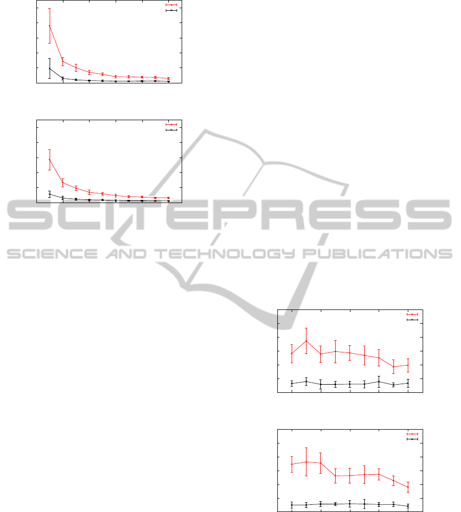
4.3 Node Density
In this experiment, p, W and Q are set to be their de-
fault values. We vary the total number of deployed
nodes, N, from 200 to 800, with the increment be-
ing 100. The results for uniform distribution and grid
distribution are shown in Figures 5(a) and (b), respec-
tively.
As we can see that as N increases, the network
lifetime of both no-recovery scheme and the recovery
scheme decreases. For no-recovery scheme, this trend
is anticipated. For uniform distribution in a given de-
ployment field, the number of nodes that reside within
0
50
100
150
200
250
300
350
100 200 300 400 500 600 700 800 900
Network lifetime (rounds)
Total number of nodes
uniform_recovery
uniform_no_recovery
(a) Uniform Distribution
0
50
100
150
200
250
300
350
100 200 300 400 500 600 700 800 900
Network lifetime (rounds)
Total number of nodes
grid_recovery
grid_no_recovery
(b) Grid Distribution.
Figure 5: Network lifetime vs. N.
the query area, N
in
, is proportional to the total number
of nodes and the percentage of the deployment field
covered by the query: N
in
= N × Q. For grid distribu-
tion, the previously indicated relations holds true ap-
proximately. As shown in the equation for P
f
, when
N
in
increases, P
f
increases monotonically, which re-
sults in a lower expected value of E[L]. Thus, the first
node failure is expected to happen earlier when the
network becomes denser.
For the recovery scheme, the average number of
neighbors N
nb
increases as the network gets denser.
For uniform distribution, N
nb
increases linearly with
N and for grid distribution it increases monotonically
with N.
Similar to the discussion in Section 4.2 , a larger
N
nb
can not guarantee a longer lifetime for the recov-
ery scheme since each recovery candidate has a less
likelihood to be valid. According to the equation for
P
v
, a larger N
nb
yields a smaller P
v
. However, the drop
of P
v
is not the only reason why the recovery candi-
dates are less likely to be considered as valid. Note
P
v
of different recovery candidates can not be consid-
ered as independent. As the network becomes denser,
there is a greater chance that two or more recovery
candidates share some neighboring nodes in common.
Once a common node fails, all the associated recovery
candidates are considered as invalid and therefore can
not be used to initiate the recovery process. Consider
the example in Figure 6.
Assume we are trying to recovery node 1. Node
1 has two recovery candidates: node 3 and node 4,
which share the same neighboring node 7. Should
RAID'ingWirelessSensorNetworks-DataRecoveryforNodeFailures
305

D6 P6
D5 P5
D3 P3
D1 P1
D4 P4 D2 P2
D7 P7
Figure 6: An example of common node shared by recovery
candidates.
node 7 have failed, neither node 3 nor node 4 could be
considered as a valid candidate for the recovery. The
denser the network is, the more likely that this sce-
nario can be observed. Thus, apart from the decrease
of P
v
, recovery candidates are less likely to meet the
requirements of valid candidates as the network den-
sity increases.
4.4 Query Size
Since our definition of network lifetime is associated
with observed node failures within a given query area,
one may question whether the size of the query area
matters to the outcome. In this experiment, we vary
the percentage of the deployment field that is covered
by the query from 5% to 30%. The other parameters
are set to their default values.
0
50
100
150
200
250
300
0 5 10 15 20 25 30 35
Network lifetime (rounds)
Percentage of the deployment field covered by the query (%)
uniform_recovery
uniform_no_recovery
(a) Uniform Distribution
0
50
100
150
200
250
300
0 5 10 15 20 25 30 35
Network lifetime (rounds)
Percentage of the deployment field covered by the query (%)
grid_recovery
grid_no_recovery
(b) Grid Distribution.
Figure 7: Network lifetime vs. Q.
From Figure 7, we can see that the network
lifetime of both recovery scheme and no-recovery
scheme decreases as Q increases and the other pa-
rameters are kept constant. Clearly N
in
increases as
we enlarge Q. Therefore, the network lifetime of no-
recovery scheme is expected to decrease since the first
node failure is expected to come earlier, as per P
f
and
E[L]. For the recovery scheme, given this parameter
setting where N
nb
and p are fixed, the total number
of recovery candidates and P
v
for each recovery can-
didate will not be affected by the query size. Thus,
the probability that each node failure is recoverable
stays the same no matter how the query size varies.
However, as N
in
increases, the probability that all the
nodes are recoverable decreases. Thus, the first non-
recoverable node failure is expected to happen earlier
and a shorter network lifetime is observed for the re-
covery scheme when Q increases.
4.5 Communication Overhead
Our scheme clearly imposes an overhead in term of
energy cost, due to the need to update a node’s neigh-
bor proactively, so that the node recovery can take
place. In the experiments above, in order to iso-
late side-effects due to energy constraints and conse-
quently better evaluate the pros and cons of our pro-
posal in terms of data recoverability, we assumed that
there was enough initial energy available that no node
run out of energy during a simulation. We now drop
this constraint.
In order to investigate our proposal’s energy over-
head we compared the total energy cost of E
upd
and
E
que
. E
rec
was ignored since the other two compo-
nents are typically one to two orders of magnitude
greater than E
rec
and p, W , N, Q were all set to be
default values. We summed up the accumulative en-
ergy cost of E
upd
and E
que
till the network lifetime of
the proposed scheme ends. We observed that the total
E
upd
was approximately 4 times as expensive as the
total E
que
on average. A legitimate question at this
point is the following: given this energy cost over-
head, does a WSN using our proposed scheme actu-
ally function for a longer time so that it is worthwhile,
compared to the no-recovery scheme? The answer is
affirmative.
Recall that we define end of WSN’s lifetime as
the point in time where it can no longer recover node
from a failed node. That is, even though all non-failed
nodes may still have energy the WSN is effectively
not as useful as queries will report incorrect answers.
In the following we will show that, given the same
amount of initial energy supply to all nodes, in most
cases a WSN without our recovery scheme will cease
to be useful earlier than any node depletes its energy
source when using our recovery scheme. In other
SENSORNETS2014-InternationalConferenceonSensorNetworks
306

words, the energy overhead is worth in the sense that
it prolongs the useful lifetime of the WSN.
Let us now investigate how different initial en-
ergy supply levels affect the performance of the re-
covery scheme and no-recovery scheme. The param-
eters, p, W , N, and Q were all set to be their default
values. We set the range of initial energy supply per
node to be [5mJ, 50mJ]. This setting is pessimistic in
the sense that batteries would typically have a much
larger charge
3
making the energy overhead of our ap-
proach be even less noticeable when compared to the
inherent probability of failure. The cause of a node
failure is two-fold: either due to energy depletion or
due to the node failure probability p. The network
lifetime achieved for uniform distribution and grid
distribution is presented in Figures 8(a) and (b), re-
spectively.
0
50
100
150
200
250
0 10 20 30 40 50
Network lifetime (rounds)
Initial energy supply per node (mJ)
uniform_recovery
uniform_no_recovery
(a) Uniform Distribution
0
50
100
150
200
250
0 10 20 30 40 50
Network lifetime (rounds)
Initial energy supply per node (mJ)
grid_recovery
grid_no_recovery
(b) Grid Distribution.
Figure 8: Network lifetime vs initial energy budgets.
For both distributions, different levels of initial
energy supply do not affect the network lifetime for
our no-recovery scheme. The moment that the first
node failure takes place, which is considered as the
termination of network lifetime for the no-recovery
scheme, the sensors have yet not suffered from energy
depletion in the vast majority of cases, even when
the initial energy supply per node is as low as 5mJ.
Thus, the node failure resulting from energy depletion
can barely affect the network lifetime for no-recovery
scheme. The trend of network lifetime is therefore the
same as if there were no energy constraint.
3
http://www.allaboutbatteries.com/Energy-tables.html
For the recovery scheme, when the initial energy
supply varies in the range of [5mJ, 20mJ], decreas-
ing the initial energy supply can shorten the network
lifetime. In this range, sensors typically run out of
energy before the first node failure caused by p takes
place, resulting in an early termination of the “useful”
network lifetime. However, when sensors are initially
charged with as little as 20mJ, the energy can usually
last longer than the first non-recoverable node failure
caused by p. Thus, varying the initial energy supply
in the range above 20mJ, which is a quite reasonable
assumption, will have very limited impact on the net-
work lifetime.
5 CONCLUSIONS
We proposed a fault recovery scheme to recover the
data after node failures take place in WSNs. Our
scheme is suitable for WSN applications where the
system designer is willing to pay for some commu-
nication overhead in exchange for higher data avail-
ability. Inspired by the RAID 4 technique for redun-
dancy of hard disks, we designed the recovery scheme
in a generic way so that it can be integrated with other
WSN protocols/algorithms.
We conducted a series of experiments to show
the network lifetime gain of the proposed recovery
scheme under different parameters: node failure prob-
ability, communication range, node density and query
size. Even in the worst case scenario, the network
lifetime of the proposed scheme can still achieve at
least three times as long as the lifetime of no-recovery
scheme. In addition, we have shown that the commu-
nication overhead imposed by our approach pays off
in the sense that a WSN using our proposed scheme
will last longer (in terms of usefulness) than a “plain”
WSN.
While out work focuses on recovering data due
to node failures, it assumes that all the message
transmissions are reliable. In fact, messages can
be dropped due to the interference caused by either
environmental noise or message collisions at sensor
nodes. Thus, a mechanism to improve the transmis-
sion reliability that can be seamlessly integrated into
our framework would be an interesting venue for fur-
ther work. Erasure coding (Wang et al., 2005) may be
an option to achieve such goal.
ACKNOWLEDGEMENTS
Research partially supported by NSERC Canada.
RAID'ingWirelessSensorNetworks-DataRecoveryforNodeFailures
307

REFERENCES
Alwan, H. and Agarwal, A. (2009). A survey on fault tol-
erant routing techniques in wireless sensor networks.
Proc. of the 3rd Intl. Conf. on Sensor Technologies and
Applications, pages 366–371.
Chessa, S. and Maestrini, P. (2005). Fault recovery mecha-
nism in single-hop sensor networks. Computer Com-
munications, 28(17):1877–1886.
Coman, A., Sander, J., and Nascimento, M. A. (2005). An
analysis of spatio-temporal query processing in sen-
sor networks. In Proc. of the 21st Intl. Conf. on Data
Engineering (Workshops), pages 1190–1195.
Dietrich, I. and Dressler, F. (2009). On the lifetime of wire-
less sensor networks. ACM Transactions on Sensor
Networks, 5(1):1–39.
Du, W., Mieyeville, F., and Navarro, D. (2010). Modeling
energy consumption of wireless sensor networks by
SystemC. In Proc. of the 5th Intl. Conf. on Systems
and Networks Communications, pages 94–98.
Ganesan, D. et al. (2001). Highly-resilient, energy-efficient
multipath routing in wireless sensor networks. ACM
SIGMOBILE Mobile Computing and Communica-
tions Review, 5(4):11–25.
Heinzelman, W. R. (2000). Application-specific protocol
architectures for wireless networks. PhD thesis, Mas-
sachusetts Institute of Technology.
Karlof, C., Li, Y., and Polastre, J. (2003). ARRIVE: Al-
gorithm for Robust Routing in Volatile Environments.
Technical report, University of California, Berkeley.
Liang, W. and Liu, Y. (2007). Online data gathering
for maximizing network lifetime in sensor networks.
IEEE Transactions on Mobile Computing, 6(1):2–11.
Marti, S. et al. (2000). Mitigating routing misbehavior
in mobile ad hoc networks. In Proc. of the 6th an-
nual Intl. Conf. on Mobile computing and networking,
pages 255–265.
Patterson, D. A., Gibson, G., and Katz, R. H. (1988). A case
for redundant arrays of inexpensive disks (RAID). In
Proc. of the 1988 ACM SIGMOD Intl. Conf. on Man-
agement of data, pages 109–116.
Rappaport, T. S. (1996). Wireless communications - princi-
ples and practice. Prentice Hall.
Shnayder, V. et al. (2004). Simulating the power consump-
tion of large-scale sensor network applications. In
Proc. of the 2nd Intl. Conf. on Embedded networked
sensor systems, pages 188–200.
Wang, Y. et al. (2005). Erasure-coding based routing for
opportunistic networks. In Proc. of the 2005 ACM
SIGCOMM workshop on Delay-tolerant networking,
pages 229–236.
Zhang, H. and Shen, H. (2009). Balancing energy consump-
tion to maximize network lifetime in data-gathering
sensor networks. IEEE Transactions on Parallel and
Distributed Systems, 20(10):1526–1539.
APPENDIX
(Patterson et al., 1988) proposed the so-called RAID
technique to solve the bottleneck issue of I/O perfor-
mance in order to catch up with the increasing speed
of CPUs and memories. Nowadays, RAID is typi-
cally referred to as a storage virtualization technol-
ogy that can replicate and distribute data among an
array of disk drives while being accessed by the oper-
ating systems as one single logical drive. Depending
on different reliability and performance requirements,
RAID can be categorized into several “levels” which
specify how the data is accessed and how the redun-
dancy is maintained. In our work, we choose the level
RAID 4 to incorporate data redundancy and achieve
fault recovery since it strikes a balance between space
efficiency and data redundancy. This level can toler-
ate at most one physical disk failure. Figure 9 shows
the diagram of a sample RAID 4 array.
parity calculation
Data disk A
Data disk B
Data disk C
Parity disk
A1
A2
A3
A4
B1
B2
B3
B4
C1
C2
C3
C4
P1
P2
P3
P4
Figure 9: RAID 4 with three data disks and one parity disk.
RAID 4 is often referred to as a dedicated par-
ity scheme since it utilizes a single disk for storing
the parity information only. In this figure, each row
within the disk represents a data block. The data
block of the parity disk stores the parity results for
all the data blocks on the data disks that are in the
same row. Denote the parity calculation as ⊕, for
data block i, within this array we have the follow-
ing relations: P
i
= A
i
⊕ B
i
⊕ C
i
. Whenever a write
is performed on any of the data disks, the parity cal-
culation component recalculates and updates the cor-
responding blocks on the parity disk. Should any of
the data disk fails, the remaining data disks, together
with the parity disk, can be utilized to reconstruct the
data of the failed disk. For instance, if data disk A
fails, we can recover its data according by computing
A
i
= P
i
⊕ B
i
⊕C
i
.
SENSORNETS2014-InternationalConferenceonSensorNetworks
308
