
Photo Rating of Facial Pictures based on Image Segmentation
Arnaud Lienhard, Marion Reinhard, Alice Caplier and Patricia Ladret
GIPSA-lab, Grenoble University, 11, rue des Mathematiques, Grenoble, France
Keywords:
Aesthetic Image Quality, Portrait, Categorization, Image Segmentation.
Abstract:
A single glance at a face is enough to infer a first impression about someone. With the increasing amount
of pictures available, selecting the most suitable picture for a given use is a difficult task. This work focuses
on the estimation of the image quality of facial portraits. Some image quality features are extracted such
as blur, color representation, illumination and it is shown that concerning facial picture rating, it is better to
estimate each feature on the different picture parts (background and foreground). The performance of the
proposed image quality estimator is evaluated and compared with a subjective facial picture quality estimation
experiment.
1 INTRODUCTION
The development of digital cameras enable people to
have access to a constantly growing number of pho-
tos. Besides, selecting good-looking images is impor-
tant in a world where everybody is constantly look-
ing at others pictures. Social psychology studies show
that a 100 milliseconds exposure time to a facial por-
trait is sufficient for people to appraise the subject at-
tractiveness, trustworthiness, competence or aggres-
siveness (Willis and Todorov, 2006).
The choice of a good facial picture may be ap-
plication dependent. Profile pictures on social net-
works are different from pictures selected in a pro-
fessional purpose. Thus, the features used for auto-
matic aesthetic scoring have to be adapted to the con-
sidered application. Aesthetic rules depend on im-
age composition, and evaluating a landscape is differ-
ent from judging a portrait, where the viewer focuses
on the subject’s face. That is why finding faces and
their contours is important for good estimation per-
formance in portraiture aesthetics.
This work demonstrates the relevance of portraits
segmentation in the case of aesthetic scoring, by com-
paring the performance of a set of features computed
either on the entire image or separately on the seg-
mented image. Performance is measured and com-
pared with the results of a subjective quality estima-
tion experiment.
1.1 Related Work
Most of articles dealing with automatic photo rating
rely on machine learning techniques. Generally, the
whole process is the following. A dataset of pic-
tures rated by humans is created, in order to obtain
the ground truth. Then, a set of features is extracted
from these pictures. Features are related to photo-
graphic rules like the rule of thirds, explain global im-
age properties like the average luminance or describe
local image properties. Finally, a learning algorithm
is performed to create an image aesthetic model us-
ing the extracted features. An example of automatic
framework for aesthetic rating of photos is presented
in (Datta et al., 2006), and is publicly available on
http://acquine.alipr.com/.
Many feature sets have been proposed and tested.
(Ke et al., 2006) focus merely on high-level fea-
tures in order to separate poor quality from profes-
sional pictures. They design features corresponding
to semantic information and abstract concepts such
as composition, color or lighting. In their approach,
(Luo and Tang, 2008) include image composition fea-
tures by separating the image into two parts: a region
with sharp edges and a blurry region. The blurry re-
gion is defined as the background, and features are
computed in both regions. However they did not focus
on portraits. Then, (Li and Gallagher, 2010) perform
face detection and include features related to human
faces and their positions: sizes, distances, etc. They
compute technical and perceptual features like con-
trast, blurring or colorfulness on both face and non
329
Lienhard A., Reinhard M., Caplier A. and Ladret P..
Photo Rating of Facial Pictures based on Image Segmentation.
DOI: 10.5220/0004673003290336
In Proceedings of the 9th International Conference on Computer Vision Theory and Applications (VISAPP-2014), pages 329-336
ISBN: 978-989-758-004-8
Copyright
c
2014 SCITEPRESS (Science and Technology Publications, Lda.)

face regions. (Khan and Vogel, 2012) adapt spatial
composition features to portraiture classification and
show the impact of the face position in aesthetic eval-
uation. However facial portraits require a more accu-
rate segmentation than only separating facial regions
from the background. For instance, hair or hats have
to be considered when evaluating the visual appeal of
a portrait.
1.2 Proposed Method
Our work focuses on frontal facial portraits, which
became very common with the proliferation of digital
cameras and social media websites.
The idea developed in this article is to show how
automatic image segmentation can improve the per-
formance of image quality evaluation. Images are
automatically segmented in 4 parts: facial skin, hair,
shoulders and background. This segmentation defines
two distinct areas. The foreground corresponds to the
subject’s face, which contains facial skin, hair, and
generally the top of the shoulders. The background
region is defined as the part of the picture which is
not the foreground. This differs from previous work,
since (Li and Gallagher, 2010) and (Khan and Vogel,
2012) only performed face detection and did not find
the precise contours of the facial regions. For estima-
tion, only few features are considered to emphasize
the importance of image segmentation. Considered
features are described in Section 3.2.
This paper is organized as follows. Section 2 de-
scribes the dataset that has been built and scored by
humans in order to have the ground truth. The quality
image features considered and the segmentation tech-
nique are explained in Section 3. Experimental results
of aesthetic quality evaluation are given in Section 4.
2 HUMAN RATING OF FACE
IMAGES
2.1 Database
A database containing 125 female and 125 male
digital pictures is considered. Half of the images
was extracted from free image datasets, such as La-
beled Faces in the Wild (Huang and Mattar, 2008)
and Caltech Face Dataset (see http://www.vision.
caltech.edu/html-files/archive.html). The other half
of facial images was acquired from private collection.
Most of them are consumer photos. They were
cropped to the extremes of the targets head and shoul-
ders (top of the head, bottom of the shoulders, sides of
hair or ears) and standardized for size (from 240×148
to 240 × 320).
The face in the picture is always right-side-up and
centered. A large variety of photos is considered: all
types of gaze and expression, facial hair styles, pres-
ence of accessories (earrings, eyeglasses, hat and vis-
ible make-up), clothing, etc.
2.2 Human Picture Rating
Twenty-five men and women, mostly aged from 20 to
30, were asked to judge facial photos using a discrete
scale from 1 (very low quality) to 6 (very high qual-
ity). They were instructed that they would be seeing
a series of faces randomly presented on a computer
screen and that their task is to assess the aesthetic
quality of each of the images displayed. Instructions
were the same for each participant: A picture will be
judged as very aesthetic when the numerous aspects
that qualify it (framing, luminosity, contrast, bloom-
ing, balance between the components, etc.) are of
good quality. Please indicate the aesthetic quality of
the picture, using a scale from 1 (very bad quality) to
6 (excellent quality).
Even if only facial portraits are considered, facial
beauty is not part of the criteria and the final objective
is to evaluate the global aesthetic quality of the picture
only.
2.3 Preliminary Results
Each image is associated with a mean score over the
25 votes and a distribution of scores corresponding
to individual votes. These scores rank from 1.36 to
5.36 (Mean of 3.21, Standard Deviation of 0.73). The
distribution is largely Gaussian and all the possible
votes are represented, as presented in Figure 1. To
estimate the reliability of the test scores, Cronbach’s
Alpha (Cronbach, 1951) is computed: α = 0.99. α
ranges between 0 and 1 and it is commonly accepted
that α > 0.9 means a very high internal consistency
of the chosen scale.
These scores are considered as the ground truth
and are used to evaluate the performance of the image
quality estimator proposed in Section 4.
3 IMAGE SEGMENTATION AND
IMAGE QUALITY FEATURES
Finding the facial skin area may help a lot for aes-
thetic scoring in portraits. Computing blur or bright-
ness values in this special location may greatly differ
VISAPP2014-InternationalConferenceonComputerVisionTheoryandApplications
330
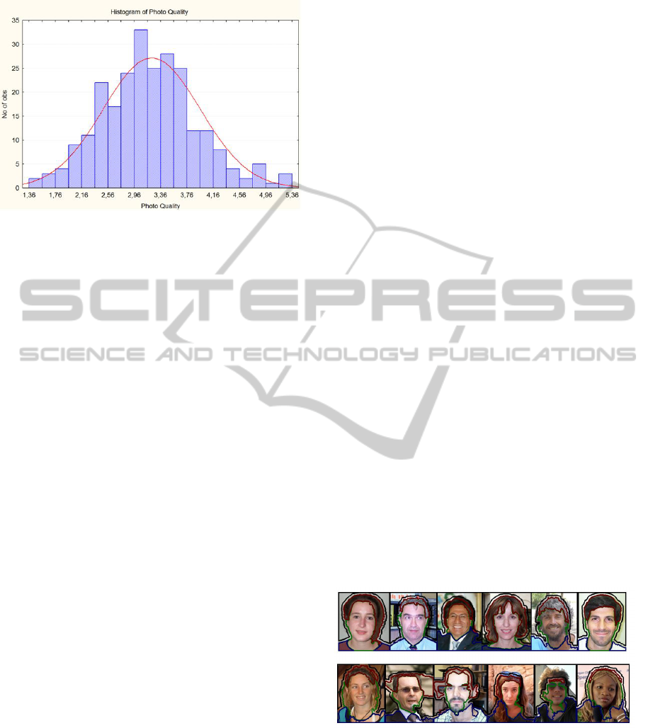
Figure 1: Histogram of image aesthetic quality mean rating.
from the global blur or brightness values, changing
our perception of the global image aesthetic.
3.1 Image Segmentation
3.1.1 Face and Facial Features Detection
Face bounding box detection is performed by using
the Viola-Jones algorithm described in (Viola and
Jones, 2001). It has been implemented in C++ us-
ing the OpenCV library, version 2.4.3. When several
faces are detected, only the biggest one is kept. De-
tection performance is good since all the faces among
the dataset of 250 images are detected.
The same algorithm is applied on the face bound-
ing box to detect eyes (left and right eyes are detected
separately), nose and mouth. Facial features detection
process has been tested on the LFW dataset (about
13,000 images) and obtained 89% of correct feature
extraction.
3.1.2 Facial Image Segmentation
The Viola-Jones algorithm provides bounding boxes
for face and facial features. Since our goal is to show
that a fine segmentation of the face is required for a
good image quality estimation, the proposed method
for face segmentation is presented below. It is based
on the results obtained after applying the Viola-Jones
algorithm.
In order to detect the location of facial contours,
the advantages of two techniques are combined (see
Figure 3). First, a histogram containing the values of
skin pixels in the area defined by the facial features
is created. After normalization, for each pixel value
in the entire image, the probability to be part of facial
skin is computed. Many skin detection models have
been developed, for example (Jones and Rehg, 1999)
used BGR color space and constructed histogram us-
ing hand labeled skin regions. Hue and saturation
channels from the HSV color space are often used.
However hue becomes less discriminant when dealing
with underexposed images or with different skin col-
ors. For that reason, red and saturation channels from
respectively BGR and HSV color spaces are used.
A segmentation algorithm is performed on the
probability image obtained from the histogram model,
to separate skin and non skin areas. Watershed is
widely used to solve segmentation problems. The
version implemented in OpenCV and inspired by
(Beucher and Meyer, 1993) is chosen. Skin area is
used as a seed for facial skin region, and image cor-
ners are used as seeds for the non skin area. Perform-
ing Watershed on the histogram back projection (see
Figure 3) prevents the algorithm from setting non skin
pixels to the facial skin area, and increases the initial
skin area defined by facial feature detection.
Using this new skin area enables us to compute a
more precise histogram, which provides a better seed
for the next iteration of segmentation. Iterating this
several times often creates fine contours. The whole
process is iterated 20 times.
To segment hair, we use exactly the same tech-
nique than for skin segmentation. The only difference
is the initialization step. Since we already have found
the skin area, and knowing that hair is above facial
skin, the area that is used to create the hair model is
defined. Same operation is done for shoulder segmen-
tation: the initial shoulder location is the image part
below facial skin region.
Finally, the background region is defined as the
remaining region, while the foreground region is the
addition of facial skin, hair and shoulders areas. Some
segmentation results are provided in Figure 2.
Figure 2: First row presents nice segmentation results,
while second row shows segmentation on more challenging
images: presence of sunglasses, unclear limitations between
skin, hair and background, etc.
3.2 Image Quality Features
6 measurements related to image quality are imple-
mented and are computed separately either in the
whole image or in subregions.
PhotoRatingofFacialPicturesbasedonImageSegmentation
331

Figure 3: Presentation of the segmentation process.
3.2.1 Blur
Blurry images are generally correlated to poor quality.
However this is not completely true with portraits: if
the face contains sharp edges, the background may be
blurred without affecting the global image aesthetic
quality. It may even enhance the visual appeal of the
picture, by increasing the contrast between face and
background.
The blur value is computed using the procedure
described in (Crete and Dolmiere, 2007). It is close
to 0 for a sharp image, and close to 1 for a blurred
image. The idea is to blur the initial image and to
compare the intensity variation of neighboring pixels
in both initial and blurred images. Figure 4 briefly
describes the blur estimation principle. A couple of
images and their blur values are presented in Figure
5.
Figure 4: Simplified flowchart of the blur estimation princi-
ple described in (Crete and Dolmiere, 2007).
Figure 5: Examples of high and low blur levels, computed
in the entire image. Blur from left to right: F
b
= 0.29 and
F
b
= 0.62. Ground truth quality scores are 4.4 and 2.0, re-
spectively.
3.2.2 Color Count
The number of colors in an image may have an impact
on the global aesthetic feeling. Figure 6 shows exam-
ple of images with high and low colorfulness values.
Many articles use hue counts (Ke et al., 2006) or the
number of colors represented in the RGB color space
(Luo and Tang, 2008). We chose to use the Lab color
space, since it is designed to approximate human vi-
sion, and the color channels (a and b) are separated
from the luminance channel (L).
A 2-dimensional histogram H is computed from
both color channels, using 16 × 16 bins. We do not
take into account pixels with too low or too high lu-
minance values L (L < 40 or L > 240), since their
color values are not significant. The histogram is nor-
malized in order to have a maximum value of 1. Let
H(i, j) be the frequency of pixels such that the a and
b color values belong to bins i and j, respectively.
We define |C| as the number of pairs (i, j) such that
H(i, j) > α. α is set to 0.001. The color count is fi-
nally:
F
c
= |C|/256 × 100% (1)
F
c
equals to 1 when all the possible colors are repre-
sented, and is close to 0 otherwise.
Figure 6: Pictures with many different colors have a higher
colorfulness value than pictures with a uniform background.
From left to right: F
c
= 0.11 and F
c
= 0.02. Ground truth
quality scores are 3.4 and 2.0, respectively.
3.2.3 Illumination and Saturation
Professional photographers often adapt the brightness
of a picture, and make the face illumination differ-
VISAPP2014-InternationalConferenceonComputerVisionTheoryandApplications
332

ent from the background enlightening. The overall
brightness should neither be too high nor too low. In
this work, brightness average and standard deviation
are considered. Computing these feature values can
be done by considering the value channel V from the
HSV color space.
The same operation is done for the saturation
channel S. Saturation is a color purity indicator. Sat-
uration average and standard deviation are computed
from the saturation channel of the HSV color space.
After computation, the following values are ob-
tained:
• µ
V
, brightness mean
• σ
V
, brightness standard deviation
• µ
S
, saturation mean
• σ
S
, saturation standard deviation
3.2.4 Final Feature Set
The final set of measurements F is
F = (F
b
,F
c
,µ
V
,σ
V
,µ
S
,σ
S
)
This measurements are computed in the 6 following
regions:
1. Entire image
2. Foreground: addition of skin, hair and shoulders
3. Background
4. Facial skin area
5. Hair area
6. Shoulders area
This makes a total of 6 × 6 features. In the experi-
ments, the feature set F
i
is the set F computed on the
region i. For example, F
1
represents the set of fea-
tures F evaluated on the entire image.
4 AUTOMATIC AESTHETIC
QUALITY ESTIMATION
In this section, classification and image scoring are
performed to show how much segmentation improves
the quality evaluation. Feature are tested separately
in section 4.2. In all the experiments, results are com-
pared with ground truth scores. 3 feature set combi-
nations are used to show segmentation influence:
1. Feature set F
1
is used to have an idea of the global
features performance, when they are computed on
the entire image.
2. Feature sets F
2
(foreground) and F
3
(background)
are used to demonstrate the segmentation influ-
ence.
3. Finally, feature sets F
3
(background), F
4
(face),
F
5
(hair) and F
6
(shoulders) are used to show the
performance improvements when the foreground
is separated in 3 parts.
We used the k-fold cross validation technique,
with k = 10. Images were removed when we could
not extract all of the facial features (e.g. images with
large sunglasses).
4.1 Influence of Segmentation on
Classification
The main objective of picture classification is to sepa-
rate good looking images from bad pictures. Support
vector machines (SVM) are widely used to perform
categorization applied to image aesthetic evaluation
(Datta et al., 2007). To classify the pictures in several
groups, SVM with a Gaussian Kernel is performed.
Performance is evaluated by the Cross-Category Er-
ror (CCE)
CCE
i
=
1
N
t
N
t
∑
n=1
I( ˆc
n
− c
n
= i)
and the Multi-Category Error (MCE)
MCE =
N
c
−1
∑
i=−(N
c
−1)
|i|CCE(i)
where N
t
is the number of test images, N
c
the number
of classes, ˆc
n
the ground truth classification described
in Section 2.3, c
n
the predicted classification. i is the
difference between ground truth and predicted classi-
fication and I(.) is the indicator function.
Since random training and testing sets are used,
and due to the limited amount of images available
in the dataset, all of the experiments are repeated 10
times with various sets. Then, the average perfor-
mance is displayed.
4.1.1 2-Class Classification
2-class categorization is used to separate high and low
quality images. Images below the median aesthetic
ground truth score are labeled as group 0, and im-
ages above as group 1. The median aesthetic score
is around 3.2 (see Figure 1). Results of the 3 exper-
iments described in Section 4 are presented in Table
1.
It has to be noticed that results are significantly above
the performance of a random classifier. Results show
that segmenting the image can help a lot to classify
PhotoRatingofFacialPicturesbasedonImageSegmentation
333

Table 1: Experimental results for 2-class categorization.
CCE
−1
is the number of overrated images, CCE
0
is the
number of good classification and CCE
1
is the number of
underrated images. Performance is the good classification
rate.
F. sets Perf. CCE
−1
CCE
0
CCE
1
F
1
75.2% 22 128 20
F
2
, F
3
77.7% 23 132 15
F
3
...F
6
83.7% 20 141 9
images in two categories. After segmentation the
good classification rate increases from 75% to almost
84%.
4.1.2 3-Class Classification
3-Class categorization is an interesting problem, since
we often want to separate highly rated or remove
poorly rated images. For this task, 3 groups of about
50 images are used. The first group contains the
50 lowest aesthetic score, the second group contains
images with medium aesthetic score (between 3 and
3.4). The last group contains only high-rated images.
We are using a total of 160 images. Images have label
0 for low aesthetic quality, 1 for medium quality and
2 for high quality.
The same experiments are conducted, and classi-
fication performance is presented in Table 2.
Table 2: Experimental results for 3-class categorization.
MCE measures the number of misclassifications.
F. sets Performance MCE
F
1
54.3% 85
F
2
, F
3
58% 80
F
3
...F
6
60.0% 78
A random classifier would have a correct classifica-
tion rate of about 33%. Again, segmentation helps for
3-Class categorization, since performance increases
from 54% to 60% after segmentation.
4.2 Influence of Image Quality Features
To have an idea of features influence, 2-Class cate-
gorization is performed using only one feature at a
time. Classification performance is reported in Table
3 for the 6 features evaluated on the entire image (F
1
),
the foreground region (F
2
) and the background region
(F
3
).
The ground truth quality score is highly correlated
with the blur value F
b
: there is about 70% of correct
classification for the dataset considered. This score
change with respect to the image region considered.
The blur value is more discriminant when computed
on the foreground region (71%, and only 66% for the
Table 3: Features good classification rates (%).
F. set F
b
F
c
µ
V
σ
V
µ
S
σ
S
F
1
70 52 55 59 54 51
F
2
71 50 57 52 57 51
F
3
66 44 49 55 50 51
background region), which is the most important part
of a portrait and should not be blurry. It is almost
the performance obtained by using the entire set F
1
(75%).
Other features like the color count F
c
or the sat-
uration standard deviation σ
S
have lower good clas-
sification rates, with respectively 52 and 51% when
computed on the entire image, which is not signifi-
cantly higher than the 50% obtained using a random
classifier.
In a portrait, a nice illumination for the subject
is important and face illumination has an impact on
image quality: the brightness mean µ
V
computed on
the foreground region has a good classification rate of
57%. The same feature evaluated on the background
region has a lower score of 49%.
4.3 Influence of Segmentation on Image
Quality Scoring
In this section, the results of quality scoring with
and without image segmentation are presented. To
this end, a Support Vector Regression (SVR) is per-
formed. All of the images available in the dataset are
used: 90% for learning and 10% for testing. An SVR
implementation is given in the OpenCV library.
Measuring the regression performance is slightly
more difficult. A model which always predicts the
average value will have a nice mean error if many im-
ages have aesthetic scores close to this mean. After
regression, the predicted data should be as close as
possible to the expected values.
To measure prediction performance, 3 criteria are
used. The Mean Squared Error E quantifies the differ-
ence between ground truth and predicted scores. Let
ˆs
n
be the ground truth and s
n
the predicted score of
picture n:
E =
1
N
t
N
t
∑
n=1
( ˆs
n
− s
n
)
2
The Pearson correlation R is defined as
R =
N
t
∑
n=1
( ˆs
n
−
¯
ˆs) · (s
n
− ¯s)
s
N
t
∑
n=1
( ˆs
n
−
¯
ˆs)
2
·
s
N
t
∑
n=1
(s
n
− ¯s)
2
VISAPP2014-InternationalConferenceonComputerVisionTheoryandApplications
334
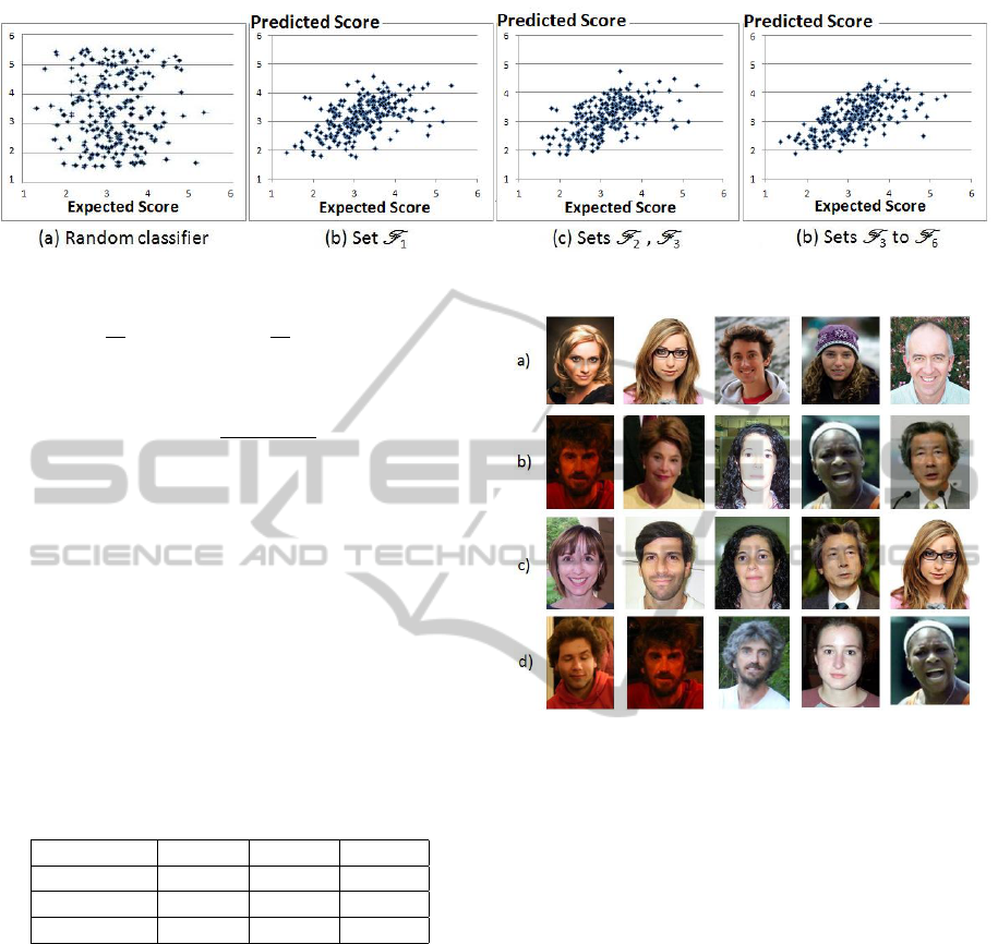
Figure 7: Prediction results for segmented and non segmented images.
where
¯
ˆs =
1
N
t
N
t
∑
n=1
ˆs
n
and ¯s =
1
N
t
N
t
∑
n=1
s
n
. Finally the
Spearman rank correlation ρ is computed
ρ = 1 −
6
∑
N
t
n=1
d
2
n
N
t
(N
2
t
− 1)
where d
n
= ˆs
n
−s
n
is the rank difference between vari-
ables. While Pearson’s measure quantifies how much
the data are linearly correlated, Spearman’s rank cor-
relation tells if the data are monotonically correlated.
Values close to 1 result from correlated data and 0
means that the data are not correlated.
Figure 7 shows the prediction results after exper-
iments and Table 4 displays the 3 coefficients com-
puted from the 3 experiments. An additional graph
is presented to show the result of a random computa-
tion. A perfect prediction would have only points on
the line y = x.
Table 4: Experimental results of regression.
Experiment Error E Corr. R Corr. ρ
F
1
0.59 0.52 0.53
F
2
, F
3
0.58 0.55 0.56
F
3
...F
6
0.55 0.61 0.64
Without any segmentation (Figure 7 b), the regres-
sion results are a lot better than randomized predic-
tion. However high and low scores may be far from
ground truth. Since the more common usages of aes-
thetic scoring are either eliminating low quality im-
ages or selecting high quality images, this is not a
satisfying result. Segmentations (Figures 7 c and d)
don’t reduce a lot the mean squared error (from 0.59
to 0.55, but reduce errors for extremes scores.
Image segmentation increases the correlation co-
efficients values from about 0.5 to 0.6: the prediction
is more accurate. Examples of very high and very low
quality images are presented in Figure 8 with their
ground truth and predicted scores.
Figure 8: a) Highest ground truth scores. b) Lowest ground
truth scores. c) Highest predicted scores. d) Lowest pre-
dicted scores.
4.4 Validation on a Larger Dataset
In order to check the robustness of the method, we
have been looking for a larger dataset, containing
frontal facial images. Many photo sharing portals ex-
ist, like Photo.net or DPChallenge.com. These web-
sites allow people to share pictures and to score oth-
ers pictures. Datasets have been created by extract-
ing such images with their scores. We chose to ex-
tract a subset of the AVA database presented in (Mur-
ray, 2012), containing 250,000 images extracted from
DPChallenge. About 800 coloured frontal facial im-
ages were found, as described in Section 2.1.
To compare with the previous experiments, 2-
class categorization is performed using the 250 im-
ages with the lowest and highest aesthetic scores. Re-
sults are presented in Table 5.
Again, good classification rate increases after seg-
mentation, from 55 to 63%. We still have interest-
ing results with simple features. However results are
worse than for the previous dataset. This may be ex-
plained by the use of more sophisticated photography
PhotoRatingofFacialPicturesbasedonImageSegmentation
335

Table 5: Experimental results for 2-class categorization of
the second dataset (500 images).
F. sets Perf. CCE
−1
CCE
0
CCE
1
F
1
55.3% 110 275 115
F
2
, F
3
58.6% 99 294 107
F
3
...F
6
63.0% 98 315 87
techniques in this dataset, making the features less ef-
fective. Moreover, it contains almost no blurry images
and performing 2-class categorization using only the
blur value computed on the foreground region leads to
an average performance of only 52.3% (71% for the
previous dataset). Pictures have a lower score vari-
ance (0.75 on a 1 to 10 scale) which makes the cate-
gorization difficult.
5 CONCLUSIONS
In this work we proposed a method based on im-
age segmentation to explore aesthetics in portraits. A
few features were extracted, and image segmentation
techniques improved evaluation performance in both
categorization and score ranking tasks.
In the experiments, only a couple of hundred im-
ages have been used and it is not sufficient to cre-
ate accurate models, especially for aesthetic scoring.
Gathering more images from different sharing portals
and other datasets may help a lot.
The features described and computed are simple
descriptors. They can be combined with generic im-
age descriptors, other data related to portraits, etc. Fa-
cial features like hair color, background composition
and textures, make-up and facial expressions, as well
as presence of hats and glasses can be used to provide
more accurate scoring.
Implementing new relevant features will be part
of future work. Comparison between several learning
techniques will be performed and additional regions
explored (e.g. eyes and mouth locations).
This will be a first step in evaluating facial por-
traits with respect to other criteria like attractiveness,
competence, aggressiveness.
REFERENCES
Beucher, S. and Meyer, F. (1993). The morphological ap-
proach to segmentation: the watershed transforma-
tion. Mathematical Morphology in Image Processing,
pages 433–481.
Crete, F. and Dolmiere, T. (2007). The blur effect: percep-
tion and estimation with a new no-reference percep-
tual blur metric. Proc. of the SPIE, 6492.
Cronbach, L. (1951). Coefficient alpha and the internal
structure of tests. Psychometrika, 16(3).
Datta, R., Joshi, D., Li, J., and Wang, J. Z. (2006). Studying
Aesthetics in Photographic Images Using a Computa-
tional Approach. ECCV, pages 288–301.
Datta, R., Li, J., and Wang, J. Z. (2007). Learning the
consensus on visual quality for next-generation image
management. Proc. of the 15th international confer-
ence on Multimedia, pages 533–536.
Huang, G. and Mattar, M. (2008). Labeled faces in the wild:
A database for studying face recognition in uncon-
strained environments. Workshop on Faces in ’Real-
Life’ Images: Detection, Alignment, and Recognition,
pages 1–11.
Jones, M. and Rehg, J. (1999). Statistical color models with
application to skin detection. CVPR, 1:274–280.
Ke, Y., Tang, X., and Jing, F. (2006). The design of high-
level features for photo quality assessment. CVPR,
1:419–426.
Khan, S. and Vogel, D. (2012). Evaluating visual aesthetics
in photographic portraiture. Proc.of the Eighth Annual
Symposium on Computational Aesthetics in Graphics,
Visualization, and Imaging (CAe ’12), pages 1–8.
Li, C. and Gallagher, A. (2010). Aesthetic quality assess-
ment of consumer photos with faces. ICIP, pages
3221 – 3224.
Luo, Y. and Tang, X. (2008). Photo and video quality eval-
uation: Focusing on the subject. ECCV, pages 386–
399.
Murray, N. (2012). AVA: A large-scale database for aes-
thetic visual analysis. CVPR, 0:2408–2415.
Viola, P. and Jones, M. (2001). Rapid object detection using
a boosted cascade of simple features. CVPR, 1:511–
518.
Willis, J. and Todorov, A. (2006). Making Up Your Mind
After a 100-Ms Exposure to a Face. Psychological
Science, 17(7):592–598.
VISAPP2014-InternationalConferenceonComputerVisionTheoryandApplications
336
