A New Covariance-assignment State Estimator in the Presence of
Intermittent Observation Losses
Sangho Ko, Seungeun Kang and Jihyoung Cha
School of Mechanical and Aerospace Engineering, Korea Aerospace University, Goyang, Gyeonggi-do, 412-791, Korea
Keywords:
Covariance Assignment, Estimation, Networked Control System (NCS), Packet Loss, Riccati Difference
Equation (RDE), Algebraic Riccati Equation (ARE).
Abstract:
This paper introduces an improved linear state estimator which directly assigns the error covariance in an
environment where the measured data are intermittently missing. Since this new estimator uses an additional
information indicating whether each observation is successfully measured, represented as a bernoulli random
variable in the measurement equation, it naturally outperforms the previous type of covariance-assignment
estimators which do not rely upon such information. This fact is proved by comparing the magnitude of
the state error covariances via the monotonicity of the Riccati difference equation, and demonstrated using a
numerical example.
1 INTRODUCTION
Construction of recursivestate estimatiors in the pres-
ence of intermittent noise-alone measurements can be
traced back to the 1960s in tackling occasional data
loss in target tracking problems in space (Nahi, 1969).
The mostly used technique to cope with this data-
loss problem in the estimation process is to model
the measurement data loss using a bernoulli random
variable taking one or zero with a probability in the
measurement equation. For example, using a random
variable γ
k
∈ {0,1} whose distribution is described by
Pr{γ
k
= 1} =
¯
γ, (1a)
Pr{γ
k
= 0} = 1 −
¯
γ, (1b)
E{γ
k
} =
¯
γ, (1c)
in the state and measurement equation
x
k+1
= Ax
k
+ v
k
, (2a)
y
k
= γ
k
Cx
k
+ w
k
, (2b)
a data-loss situation is expressed as y
k
= w
k
with γ
k
=
0 and when a data is successfully observed as y
k
=
Cx
k
+ w
k
now with γ
k
= 1. Here v
k
and w
k
are the
process and measurement noises, respectively.
In many cases such as the aforementioned track-
ing problem, the value of the random variable γ
k
is
not accessible in the estimation process of the state
x
k
. Therefore the estimators used in previous research
(Nahi, 1969) and (NaNacara and Yaz, 1997) were of
the following form
ˆ
x
k+1
= A
ˆ
x
k
+ K(y
k
−
¯
γC
ˆ
x
k
) (3)
only using the expected value of γ
k
. Nahi (1969) de-
rived the minimum variance estimators and NaNacara
& Yaz (1997) introduced covariance-assignment esti-
mators using the form (3).
One of the recent application area where this
intermittent data loss problem is important is the
networked control systems (NCS) (Hespanha et al.,
2007). In NCS, control and/or mesurement signals
among sub-components within the system are tras-
ferred via a commonly accessible network instead of
using the componet-to-component connections. Nat-
urally the problems such as data packet losses and
time delays due to the network have been major re-
search topics.
One of the major differences in NCS and the pre-
vious tracking problem is the accessibility of the in-
formation on the value of γ
k
in the state estimation
process. Both in (Sinopoli et al., 2004) and (Schen-
ato et al., 2007), the optimal state estimator over lossy
networks was derived, although the interim derivation
processes were different, in which the estimators was
of the form
ˆ
x
k+1
= A
ˆ
x
k
+ γ
k
G(y
k
− C
ˆ
x
k
). (4)
Here we can use the value of γ
k
for state estimation.
Whearas the previous type of estimators (3) uses
only {y
k
}
k=1,2,3,...
for state estimation, the new form
279
Ko S., Kang S. and Cha J..
A New Covariance-assignment State Estimator in the Presence of Intermittent Observation Losses.
DOI: 10.5220/0004673902790284
In Proceedings of the 3rd International Conference on Sensor Networks (SENSORNETS-2014), pages 279-284
ISBN: 978-989-758-001-7
Copyright
c
 2014 SCITEPRESS (Science and Technology Publications, Lda.)

of estimators (4) utilize {γ
k
} as well as {y
k
}. There-
fore, we may conjecture that the optimal estimator of
the form (4) outperforms the optimal estimator of the
form (3). In this paper, we formally prove this by
comparing magnitude of the estimation error covari-
ances.
In this context, we derive a new covariance-
assignment estimtor for linear systems using the esti-
mator form (4) in the next section and, then in Section
3, prove that the new estimator performs better than
the old one (3) by comparing the magnitude of the
state error covariances represented as the two differ-
ent Riccati difference equations (RDE) resulted from
(3) and (4). For this we use the monotonicity prop-
erty of the RDE and demonstate the difference using
a numerical example in Section 4. Finally Section 5
concludes this research.
In this paper, matrices will be denoted by upper
case boldface (e.g., A), column matrices (vectors) will
be denotedby lower case boldface (e.g.,x), and scalars
will be denoted by lower case (e.g., y) or upper case
(e.g., Y). For a matrix A, A
T
and Tr{A} denote its
transpose and trace, respectively. For a symmetric
matrix P > 0 or P ≥ 0 denotes the fact that P is pos-
itive definite or positive semi-definite, respectively.
For a random vector y, E{x} denotes the expectation
of x.
2 A NEW COVARIANCE
ASSIGNMENT STATE
ESTIMATOR
Consider the state and measurement equations rep-
resented in (2) where x
k
∈ R
n
and y
k
∈ R
p
. Here
v
k
∈ R
n
and w
k
∈ R
p
are statistically independent
zero-mean sequences representing the process and the
measurement noises, respectively. The covariances of
v
k
and w
k
are represented as V > 0 and W > 0 for
all k, respectively. The noises are assumed to be mu-
tually independent and also independent of the initial
state x
0
whose mean and covariance are
¯
x
0
and X
0
,
respectively.
The random variable γ
k
, indicating the informa-
tion whether the measurement is successfully ob-
served, has the distribution characterized by (1). For
a simple development, we introduce a new random
sequence
˜
γ
k
such that
γ
k
=
¯
γ+
˜
γ
k
, (5)
and thus
E{
˜
γ
k
} = 0, (6a)
σ
2
˜
γ
, E[(
˜
γ
k
− E{
˜
γ
k
})
2
] =
¯
γ(1−
¯
γ). (6b)
Therefore, the measurement equation (2b) can be
written as
y
k
= (
¯
γ+
˜
γ
k
)Cx
k
+ w
k
. (7)
Differently from the estimator type used in the
previous literature (NaNacara and Yaz, 1997) which
does not access γ
k
, here we employ a new estimator
form (4) which uses the informaton on γ
k
. Using the
system equations (2) and the estimator (4) yields the
state estimation error
e
k
, x
k
−
ˆ
x
k
, (8)
resulting in
e
k+1
= (A− γ
k
GC)e
k
+ v
k
+ γ
k
Gw
k
. (9)
Note that the estimator (4) is unbiased if E{e
0
} = 0.
The covariancematrix of the state estimation error
vector is defined as
P
k
, E{e
k
e
T
k
} (10)
which propagates in time according to
P
k+1
= (A−
¯
γGC)P
k
(A−
¯
γGC)
T
+ G(σ
2
¯
γ
CP
k
C
T
+
¯
γW)G
T
+ V.
(11)
Rearranging and completing square yield
P
k+1
= AP
k
A
T
+ V−
¯
γG
0
k
(CP
k
C
T
+ W)G
0
T
k
+
¯
γ(G− G
0
k
)(CP
k
C
T
+ W)(G− G
0
k
)
T
,
(12)
where
G
0
k
, AP
k
C
T
(CP
k
C
T
+ W)
−1
. (13)
If the error covariance at steady state defined as
P , lim
k→∞
E{e
k
e
T
k
} (14)
exists,
P− APA
T
− V+
¯
γG
0
(CPC
T
+ W)
−1
G
0
T
=
¯
γ(G− G
0
)(CPC
T
+ W)(G− G
0
)
T
, LL
T
,
(15)
where L ∈ R
n×p
and
G
0
, APC
T
(CPC
T
+ W)
−1
. (16)
Defining a new non-singular matrix T such that
TT
T
=
¯
γ(CPC
T
+ W) (17)
yields
LL
T
= (G− G
0
)TT
T
(G− G
0
)
T
, (18)
from which we obtain, for an arbitrary orthogonal ma-
trix U with consistent size,
LU = (G− G
0
)T. (19)
Finally the filter gain becomes
G = G
0
+ LUT
−1
= APC
T
(CPC
T
+ W)
−1
+ LUT
−1
.
(20)
The developments above can be summarized as The-
orem 1:
SENSORNETS2014-InternationalConferenceonSensorNetworks
280

Theorem 1. For the linear discrete-time stochastic
system with intermittent observation losses expressed
as (2) and the state estimator form (4), a given
steady-state covariance P of state estimation error is
assignable if and only if the left-hand side of (15) is
non-negative definite with maximum rank p. In this
case, all filter gains assign this steady-state covari-
ance P are expressed as (20).
It can be easily shown that among all the steady-
state error covariances expressed as (15), the mini-
mum error covariance is attained when the filter gain
G is equal to G
0
:
Corollary 1. The minimum error covariance attain-
able using the estimator (4) is expressed as the fol-
lowing algebraic Riccati equation (ARE)
P = APA
T
+ V−
¯
γG
0
(CPC
T
+ W)G
0
T
= APA
T
+ V−
¯
γAPC
T
(CPC
T
+ W)
−1
CPA
T
(21)
with the filter gain
G = G
0
= APC
T
(CPC
T
+ W)
−1
. (22)
The minimum error covariance given by (21) can
also be modified to
P = APA
T
+ V
−
¯
γ
2
APC
T
(
¯
γ
2
CPC
T
+ σ
2
˜
γ
CPC
T
+
¯
γW)
−1
CPA
T
(23)
using the relation
¯
γ
2
+ σ
2
˜
γ
=
¯
γ
2
+
¯
γ(1−
¯
γ) =
¯
γ.
3 PERFORMANCE
COMPARISION OF
COVARIANCE-ASSIGNMENT
ESTIMATORS
This section compares the magnitudeof state error co-
variance of the state estimator (4) newly introduced in
the previous section with that of the past estimator (3)
suggested in (NaNacara and Yaz, 1997). This estima-
tor satisfies the following estimation error covariance
equation at steady state
˜
P− A
˜
PA
T
− V
= (K− K
0
)(
¯
γ
2
C
˜
PC
T
+ σ
2
˜
γ
CXC
T
+ W)(K− K
0
)
T
− K
0
(
¯
γ
2
C
˜
PC
T
+ σ
2
˜
γ
CXC
T
+ W)K
0
T
(24)
where
K
0
=
¯
γA
˜
PC
T
(
¯
γ
2
C
˜
PC
T
+ σ
2
˜
γ
CXC
T
+ W)
−1
(25)
and X , lim
k→∞
X
k
= lim
k→∞
E{x
k
x
T
k
} is the converging so-
lution of the state covariance equation
X
k+1
= AX
k
A
T
+ V. (26)
Similarly to Corollary 1, the minimum state error
covariance at steady state is expressed as the ARE
˜
P = A
˜
PA
T
+ V
− K
0
(
¯
γ
2
C
˜
PC
T
+ σ
2
˜
γ
CXC
T
+ W)K
0
T
= A
˜
PA
T
+ V
−
¯
γ
2
A
˜
PC
T
(
¯
γ
2
C
˜
PC
T
+ σ
2
˜
γ
CXC
T
+ W)
−1
C
˜
PA
T
(27)
which is obtained by plugging K = K
0
into (24).
Remark 1 (Convergence of Riccati difference equa-
tions). It is well known (Bitmead and Gevers, 1991)
that if the matrix pair

A,C

is stabilizable and
[A,V
1/2
] is detectable, the solution of a RDE con-
verges to the solution of the corresponding ARE.
Therefore the solutions of the following RDEs
˜
P
k+1
=A
˜
P
k
A
T
+ V−
¯
γ
2
A
˜
P
k
C
T
× (
¯
γ
2
C
˜
P
k
C
T
+ σ
2
˜
γ
CX
k
C
T
+ W)
−1
C
˜
P
k
A
T
,
(28)
P
k+1
=AP
k
A
T
+ V−
¯
γ
2
AP
k
C
T
× (
¯
γ
2
CP
k
C
T
+ σ
2
˜
γ
CP
k
C
T
+
¯
γW)
−1
CP
k
A
T
(29)
convergeto the solution of (27) and (23), respectively.
In order to compare the magnitude of P with
˜
P, the
followng monotonicity property of the Riccati equa-
tion (Bitmead and Gevers, 1991) is useful.
Lemma 1 (Monotonicity property #1 of the RDE
(Bitmead and Gevers, 1991)). Consider two Riccati
Difference Equations with the same A, C and R ma-
trices but possibly different V
1
and V
2
. Denote their
solution matrices P
1
k
and P
2
k
, respectively, of the fol-
lowing two Riccati difference equations
P
i
k+1
= AP
i
k
A
T
+ V
i
− AP
i
k
C
T
(CP
i
k
C
T
+ W)
−1
CP
i
k
A
T
, i = 1,2.
(30)
Suppose that V
1
≥ V
2
, and, for some k we have P
1
k
≥
P
2
k
, then for all j > 0
P
1
k+ j
≥ P
2
k+ j
. (31)
Using this Lemma 1, a similar monotonicity prop-
erty of the RDE now with different W
i
but the same
V matrix can be obtained.
Lemma 2 (Monotonicity property #2 of the RDE ).
Consider two Riccati Difference Equations with the
same A, C and V matrices but possibly different W
1
and W
2
. Denote their solution matrices P
1
k
and P
2
k
,
respectively, of the following two Riccati difference
equations
P
i
k+1
= AP
i
k
A
T
+ V
−AP
i
k
C
T
(CP
i
k
C
T
+W
i
)
−1
CP
i
k
A
T
, i = 1,2.
(32)
ANewCovariance-assignmentStateEstimatorinthePresenceofIntermittentObservationLosses
281

Suppose that W
1
≥ W
2
, and, for some k we have P
1
k
≥
P
2
k
, then for all j > 0
P
1
k+ j
≥ P
2
k+ j
. (33)
Proof 1. See Appendix.
Since X
k
≥ P
k
based on (26) and (29) and
¯
γ < 1,
we have
σ
2
˜
γ
CX
k
C
T
+ W ≥ σ
2
˜
γ
CP
k
C
T
+
¯
γW, (34)
and the difference between the two terms above is
∆
k
, σ
2
˜
γ
C(X
k
− P
k
)C
T
+ (1−
¯
γ)W
= (1−
¯
γ)(
¯
γ∇
k
+ W) ≥ 0
(35)
with ∇
k
, C(X
k
− P
k
)C
T
≥ 0.
Therefore, applying Lemma 2 to (28) and (29) to-
gether with (34) yields
˜
P
k
≥ P
k
for all k > 0, (36)
provided that each of the initial covariances are the
same.
Now if the sufficient conditions hold for the con-
vergence of the RDE in Remark 1, the following the-
orem can be obtained from (36).
Theorem 2. For the discrete-time stochastic system
with intermittent observation losses expressed as (2),
the state estimators given by (3) and (4) yield the min-
imum covariances of state estimation error (27) and
(23), respectively. Furthermore,
˜
P ≥ P, (37)
i.e., the state error covariance of the old estimator (3)
is bigger than that of the current estimator (4).
Based on Theorem 2 and (35), we observe the fol-
lowng:
(1) As we can expect, when
¯
γ = 1, there is no perfor-
mance difference between the two estimators, i.e.,
˜
P = P;
(2) Whether ∆
k
is increasing or decreasing with re-
spect to
¯
γ is not straightforward because the
derivative
∂∆
k
∂
¯
γ
= −(2
¯
γ∇
k
+ W) +

∇
k
+
¯
γ(1−
¯
γ)
∂∇
k
∂
¯
γ

(38)
can be non-negative or non-positive matrix
1
.
However, if
¯
γ and the noise covariance W are
relatively big, the derivative may become a non-
positive definite. In this case, the bigger
¯
γ the
smaller the performance difference.
1
Note
∂∇
k
∂
¯
γ
= −
∂P
k
∂
¯
γ
≥ 0 from the monotonicity prop-
erty in Lemma 1.
Remark 2 (Connections to the Kalman filter with in-
termittent observation). The Kalman filter with inter-
mittent observation derived in Refs. (Sinopoli et al.,
2004) and (Schenato et al., 2007) iterates a Riccati
difference equation:
Σ
k+1
= AΣ
k
A
T
+ V
− γ
k
AΣ
k
C
T
(CΣ
k
C
T
+ W)
−1
CΣ
k
A
T
(39)
However, the covariance obtained by this equation is
stochastic since it depends on γ
k
so that it cannot be
calculated offline. They suggested a deterministic up-
per bound of the expectation of Σ
k
:
E
γ
{Σ
k
} ≤ P
k
(40)
We observe that this upper bound is equal to the non-
steady-state version of the algebraic Riccati equation
(23) developed in this paper.
4 NUMERICAL EXAMPLE
In order to demonstrate the performance difference
between the two estimators using covariance assign-
ment as proved in the previous section, the same nu-
merical example as in (NaNacara and Yaz, 1997) is
used here:
x
k+1
=

0.90 0.02
0.01 0.84

x
k
+ v
k
(41a)
y
k
= γ
k

1 0

x
k
+ w
k
(41b)
Here the zero-mean noise sequence v
k
and w
k
have
gaussian distributions with covariaces, respectively,
V =

0.01 0
0 0.02

,
W = 0.02.
(42)
To see the effect of the observation-success prob-
ability on performance difference, two different val-
ues of
¯
γ = 0.9 and 0.6 were tried. To confirm the
result using the algebraic Riccati equations (27) and
(23), a 10000-run Monte-carlo simulation was also
conducted for each case. The followings summarize
the result of each case.
•
¯
γ = 0.9 case:
Based on the filter gains (22) and (25) for the new and
old estimators respectively
G = G
0
=

0.4348
0.0517

,
K = K
0
=

0.3880
0.0462

,
(43)
SENSORNETS2014-InternationalConferenceonSensorNetworks
282

the algebraic Riccati equations and the 10000-run
Monte-Carlo simulation result in
P
Riccati
=

0.0186 0.0022
0.0022 0.0677

,
˜
P
Riccati
=

0.0194 0.0022
0.0022 0.0678

,
(44)
and
P
Monte
=

0.0189 0.0016
0.0016 0.0702

,
˜
P
Monte
=

0.0201 0.0016
0.0016 0.0701

.
(45)
•
¯
γ = 0.6 case:
G
0
=

0.4782
0.0573

,
K
0
=

0.3223
0.0388

,
(46)
P
Riccati
=

0.0225 0.0026
0.0026 0.0678

,
˜
P
Riccati
=

0.0250 0.0029
0.0029 0.0678

,
(47)
P
Monte
=

0.0225 0.0026
0.0026 0.0678

,
˜
P
Monte
=

0.0250 0.0029
0.0029 0.0678

.
(48)
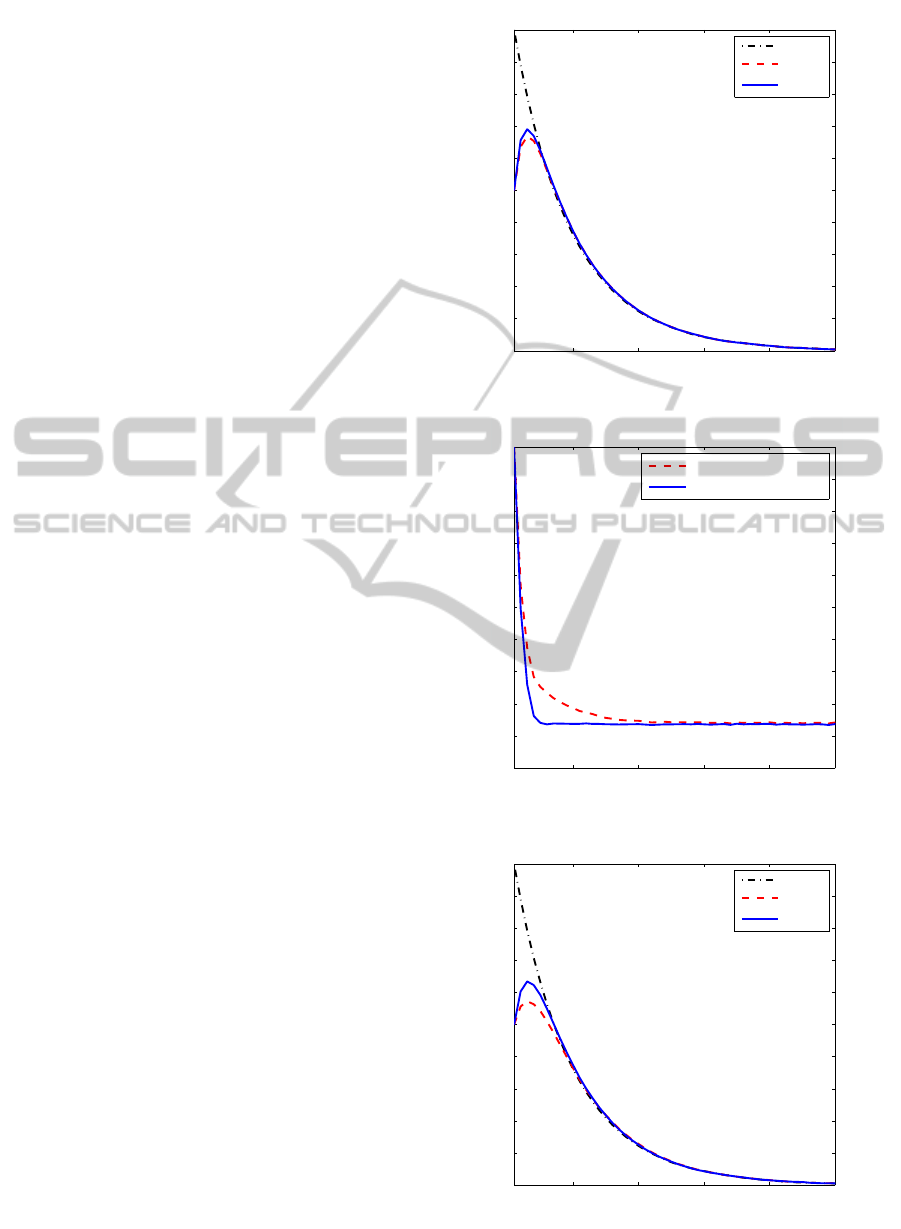
The numerical results shown above confirm the
formal verification of Section 3 that the new estima-
tor accessing the information on γ
k
outperforms the
old estimator in terms of the minimum error covari-
ance. This simulation results are also shown in Figure
1 through Figure 4. Figure 1 and 2 compare the es-
timates of the first state and the estimation errors in
terms of absolute errors for
¯
γ = 0.9. Figure 3 and 4
correspond to
¯
γ = 0.6 case. As shown the figures, the
smaller
¯
γ, the bigger the peformance difference.
5 CONCLUSIONS
This paper confirmed that in the presence of inter-
mittent observation losses the new covariance as-
signment estimator which can access the informa-
tion on observation-success or fail performs better
than the previous covariance-assignment state estima-
tor which does not use such an information. The per-
formance difference was formally shown by compar-
ing the magnitude of the error covariance matrices via
the monotonicity properties of the Riccati equation.
10 20 30 40 50
0
0.2
0.4
0.6
0.8
1
1.2
1.4
1.6
1.8
2
Time index k
x(1)
xhat
old
xhat
new
Figure 1: Comparison of state estimates with
¯
γ = 0.9.
10 20 30 40 50
0
0.1
0.2
0.3
0.4
0.5
0.6
0.7
0.8
0.9
1
Time index k
absolute error of xhat
old
absolute error of xhat
new
Figure 2: Comparison of estimation errors with
¯
γ = 0.9.
10 20 30 40 50
0
0.2
0.4
0.6
0.8
1
1.2
1.4
1.6
1.8
2
Time index k
x(1)
xhat
old
xhat
new
Figure 3: Comparison of state estimates with
¯
γ = 0.6.
ANewCovariance-assignmentStateEstimatorinthePresenceofIntermittentObservationLosses
283

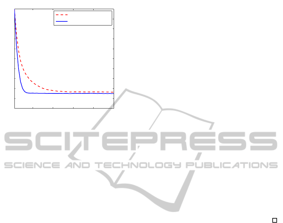
10 20 30 40 50
0
0.1
0.2
0.3
0.4
0.5
0.6
0.7
0.8
0.9
1
Time index k
absolute error of xhat
old
absolute error of xhat
new
Figure 4: Comparison of estimation errors with
¯
γ = 0.6.
This fact was then numerically demonstrated using a
discrete-time linear stochastic system example.
ACKNOWLEDGEMENTS
This research was supported by Basic Science Re-
search Program through the National Research Foun-
dation of Korea (NRF) funded by the Ministry of Ed-
ucation, Science and Technology (2011-0013998).
REFERENCES
Bitmead, R. R. and Gevers, M. (1991). Riccati difference
and differential equations: Convergence, monotonic-
ity and stability. In Bittanti, S., Laub, A. J., and
Willems, J. C., editors, The Riccati equation, pages
263–291. Springer-Verlag, Berlin, Germany.
Hespanha, J., Naghshtabrizi, P., and Xu, Y. (2007). A sur-
vey of recent results in networked control systems.
Proceedings of the IEEE, 95(1):138–162.
Nahi, N. E. (1969). Optimal recursive estimation with un-
certain observation. IEEE Transactions on Informa-
tion Theory, IT-15(4):457–462.
NaNacara, W. and Yaz, E. E. (1997). Recursive estimator
for linear and nonlinear systems with uncertain obser-
vations. Signal Processing, 62(15):215–228.
Schenato, L., Sinopoli, B., Franceschetti, M., Polla, K., and
Sastry, S. (2007). Foundations of control and estima-
tion over lossy networks. Proceedings of the IEEE,
95(1):163–187.
Sinopoli, B., Schenato, L., Franceschetti, M., Poolla, K.,
Jordan, M. I., and Sastry, S. S. (2004). Kalman filter-
ing with intermittent observations. IEEE Transactions
on Automatic Control, 49(9):1453–1464.
APPENDIX
Proof for Lemma 2
Let W
1
= W
2
+ ∆W with ∆W ≥ 0. Then using the
matrix inversion lemma yields
(CP
1
k
C
T
+ W
1
)
−1
= (CP
1
k
C
T
+ W
2
+ ∆W)
−1
= (CP
1
k
C
T
+ W
2
)
−1
− M
(49)
with
M , (CP
1
k
C
T
+ W
2
)
−1
∆W
1/2
× [∆W
1/2
(CP
1
k
C
T
+ W
2
)
−1
∆W
1/2
+ I]
−1
× ∆W
1/2
(CP
1
k
C
T
+ W
2
)
−1
≥ 0.
(50)
Then the first Riccati equation becomes
P
1
k+1
= AP
1
k
A
T
+ V
1
− AP
1
k
C
T
(CP
1
k
C
T
+ W
2
)
−1
CP
1
k
A
T
(51)
with V
1
, V+ AP
1
k
C
T
MCP
1
k
A
T
≥ V since M ≥ 0.
Comparing this with the second Riccati equation
P
2
k+1
= AP
2
k
A
T
+ V
− AP
2
k
C
T
(CP
2
k
C
T
+ W
2
)
−1
CP
2
k
A
T
(52)
yields
P
1
k+ j
≥ P
2
k+ j
. (53)
based on Lemma 1.
SENSORNETS2014-InternationalConferenceonSensorNetworks
284