
Learning a Loopy Model Exactly
Andreas Christian M¨uller and Sven Behnke
Institute of Computer Science VI, Autonomous Intelligent Systems, University of Bonn, Bonn, Germany
Keywords:
Structured Prediction, Image Segmentation, Structured SVMs, Conditional Random Fields.
Abstract:
Learning structured models using maximum margin techniques has become an indispensable tool for com-
puter vision researchers, as many computer vision applications can be cast naturally as an image labeling
problem. Pixel-based or superpixel-based conditional random fields are particularly popular examples. Typ-
ically, neighborhood graphs, which contain a large number of cycles, are used. As exact inference in loopy
graphs is NP-hard in general, learning these models without approximations is usually deemed infeasible.
In this work we show that, despite the theoretical hardness, it is possible to learn loopy models exactly in
practical applications. To this end, we analyze the use of multiple approximate inference techniques together
with cutting plane training of structural SVMs. We show that our proposed method yields exact solutions
with an optimality guarantees in a computer vision application, for little additional computational cost. We
also propose a dynamic caching scheme to accelerate training further, yielding runtimes that are comparable
with approximate methods. We hope that this insight can lead to a reconsideration of the tractability of loopy
models in computer vision.
1 INTRODUCTION
Many classical computer vision applications such as
stereo, optical flow, semantic segmentation and visual
grouping can be naturally formulated as image label-
ing tasks.
Arguably the most popular way to approach such
labeling problems is via graphical models, such as
Markov random fields (MRFs) and conditional ran-
dom fields (CRFs). MRFs and CRFs provide a prin-
cipled way of integrating local evidence and model-
ing spacial dependencies, which are strong in most
image-based tasks.
While in earlier approaches, model parameters
were set by hand or using cross-validation, more
recently parameters are often learned using a max-
margin approach. Most models employ linear energy
functions of unary and pairwise interactions, trained
using structural support vector machines (SSVMs).
While linear energy functions lead to learning prob-
lems that are convex in the parameters, complex con-
straints complicate their optimization. Additionally,
inference (or more precisely loss-augmented predic-
tion) is a crucial part in learning, and can often not be
performed exactly, due to loops in the neighborhood
graphs. Approximations in the inference then lead to
approximate learning.
We look at semantic image segmentation, learn-
ing a model of pairwise interactions on the popular
MSRC-21 and Pascal VOC datasets. The contribu-
tion of this work is threefold:
• We analyze the simultaneous use of multiple ap-
proximate inference methods for learning SSVMs
using the cutting plane method, relating approxi-
mate learning to the exact optimum.
• We introduce an efficient caching scheme to ac-
celerate cutting plane training.
• We demonstrate that using a combination of
under-generatingand exactinference methods, we
can learn an SSVM exactly in a practical applica-
tion, even in the presence of loopy graphs.
While empirically exact learning yields results
comparable to those using approximate inference
alone, certification of optimality allows treating learn-
ing as a black-box, enabling the researcher to focus
attention on designing the model for the application
at hand. It also makes research more reproducible,
as the particular optimization methods that are used
become less relevant to the result.
2 RELATED WORK
Max margin learning for structured prediction was
introduced by Taskar et al. (2003), in the form of
337
Christian Müller A. and Behnke S..
Learning a Loopy Model Exactly.
DOI: 10.5220/0004674503370344
In Proceedings of the 9th International Conference on Computer Vision Theory and Applications (VISAPP-2014), pages 337-344
ISBN: 978-989-758-004-8
Copyright
c
2014 SCITEPRESS (Science and Technology Publications, Lda.)

maximum-margin Markov models. Later, this frame-
work was generalized to structural support vector ma-
chines by Tsochantaridis et al. (2006). Both works
assume tractable loss-augmented inference.
Currently the most widely used method is the
one-slack cutting plane formulation introduced by
Joachims et al. (2009). This work also introduced the
caching of constraints, which serves as a basis for our
work. We improve upon their caching scheme, and in
particular consider how it interacts with approximate
inference algorithms.
Recently, there has been an increase in research in
learning structured prediction models where standard
exact inference techniques are not applicable, in par-
ticular in the computer vision community. The influ-
ence of approximate inference on structural support
vector machine learning was first analyzed by Fin-
ley and Joachims (2008). Finley and Joachims (2008)
showed convergence results for under-generating and
over-generating inference procedures, meaning meth-
ods that find suboptimal, but feasible solutions, and
optimal solutions from a larger (unfeasible) set, re-
spectively. Finley and Joachims (2008) demonstrated
that over-generating approaches—in particular linear
programming (LP)—perform best on the considered
model. They also give a bound on the empirical risk
for this case. In contrast, we aim at optimizing the
non-relaxed objective directly, yielding the original,
tighter bound.
As using LP relaxations was considered too costly
for typical computer vision approaches, later work
employed graph-cuts (Szummer et al., 2008) or
Loopy Belief Propagation(LBP) (Lucchi et al., 2011).
These works use a single inference algorithm during
the whole learning process, and can not provide any
bounds on the true objective or the empirical risk. In
contrast, we combine different inference methods that
are more appropriate for different stages of learning.
Recently, Meshi et al. (2010), Hazan and Urta-
sun (2010) and Komodakis (2011) introduced formu-
lations for joint inference and learning using duality.
In particular, Hazan and Urtasun (2010) demonstrated
the performance of their model on an image denois-
ing task, where it is possible to learn a large number of
parameters efficiently. While these approaches show
great promise, in particular for pixel-level or large-
scale problems, they perform approximate inference
and learning, and do not relate their results back to
the original SSVM objective they approximate.
3 EFFICIENT CUTTING PLANE
TRAINING OF SSVMs
3.1 The Cutting Plane Method
When learning for structured prediction in the max-
margin framework of Tsochantaridis et al. (2006),
predictions are made as
argmax
y∈Y
f(x,y,θ),
where x ∈ X is the input, y ∈ Y the prediction, and θ
are the parameters to be learned. We will assume y to
be multivariate, y = (y
1
,.. ., y
k
) with possibly varying
k.
The function f measures compatibility of x and y
and is a linear function of the parameters θ:
f(x, y,θ) = hθ,ψ(x,y)i.
Here ψ(x,y) is a joint feature vector of x and y. Speci-
fying a particular SSVM model amounts to specifying
ψ.
For a given loss ∆, the parameters θ are learned by
minimizing the loss-based soft-margin objective
min
θ
1
2
||θ||
2
+C
∑
i
r
i
(θ) (1)
with regularization parameter C, where r
i
is a hinge-
loss-like upper bound on the empirical ∆-risk:
r
i
(x
i
,y
i
,y) =
max
y∈Y
∆(y
i
,y) +
θ,ψ(x
i
,y) − ψ(x
i
,y
i
)
+
We solve the following reformulation of Equa-
tion 1, known as one-slack QP formulation:
min
θ,ξ
1
2
||θ||
2
+Cξ (2)
s.t. ∀
ˆ
y = ( ˆy
1
,.. ., ˆy
n
) ∈ Y
n
: (3)
*
θ,
n
∑
i=1
[ψ(x
i
,y
i
) − ψ(x
i
, ˆy
i
)]
+
≥
n
∑
i=1
∆(y
i
, ˆy
i
) − ξ
(4)
using the cutting plane method described in Algo-
rithm 1 (Joachims et al., 2009).
The cutting plane method alternates between solv-
ing Equation (2) with a working set W of constraints,
and expanding the working set using the current θ
by finding y corresponding to the most violated con-
straint, using a separation oracle I. We investigate the
construction of W and the influence of I on learning.
Intuitively, the one-slack formulation corresponds
to joining all training samples into a single training
VISAPP2014-InternationalConferenceonComputerVisionTheoryandApplications
338

Algorithm 1: Cutting Plane Training of Structural SVMs.
Require: Training samples {(x
1
,y
1
),... , (x
n
,y
n
)}, regularization parameter C, stopping tolerance ε, separation
oracle I.
Ensure: Parameters θ, slack ξ
1: W ←
/
0
2: repeat
3: (θ,ξ) ← argmin
θ,ξ
||θ||
2
2
+Cξ
4:
s.t. ∀
ˆ
y = ( ˆy
1
,.. ., ˆy
n
) ∈ W :
*
θ,
n
∑
i=1
[ψ(x
i
,y
i
) − ψ(x
i
, ˆy
i
)]
+
≥
n
∑
i=1
∆(y
i
, ˆy
i
) − ξ
5: for i=1, ..., n do
6: ˆy
i
← I(x
i
,y
i
,θ) ≈ argmax
ˆy∈Y
n
∑
i=1
∆(y
i
, ˆy) −
*
θ,
n
∑
i=1
[ψ(x
i
,y
i
) − ψ(x
i
, ˆy)]
+
7: W ← W ∪ {( ˆy
1
,.. ., ˆy
n
)}
8: ξ
′
←
n
∑
i=1
∆(y
i
, ˆy
i
) −
*
θ,
n
∑
i=1
[ψ(x
i
,y
i
) − ψ(x
i
, ˆy
i
)]
+
9: until ξ
′
− ξ < ε
example (x,y) that has no interactions between vari-
ables corresponding to different data points. Conse-
quently, only a single constraint is added in each itera-
tion of Algorithm 1, leading to very small W . We fur-
ther use pruning of unused constraints, as suggested
by Joachims et al. (2009), resulting in the size of W
being in the order of hundreds for all experiments.
We also use another enhancement of the cutting
plane algorithm introduced by Joachims et al. (2009),
the caching oracle. For each training example (x
i
,y
i
),
we maintain a set C
i
of the last r results of loss-
augmented inference (line 6 in Algorithm 1). For gen-
erating a new constraint ( ˆy
1
,.. ., ˆy
n
) we find
ˆy
i
← argmax
ˆy∈C
i
n
∑
i=1
∆(y
i
, ˆy) −
*
θ,
n
∑
i=1
[ψ(x
i
,y
i
) − ψ(x
i
, ˆy)]
+
by enumerationofC
i
and continue until line 9. Only if
ξ
′
− ξ < ε, i.e. the produced constraint is not violated,
we return to line 6 and actually invoke the separation
oracle I.
In computer vision applications, or more gener-
ally in graph labeling problems, ψ is often given as
a factor graph over y, typically using only unary and
pairwise functions:
hθ, ψ(x,y)i =
k
∑
i=0
hθ
u
,ψ
u
(x, y
k
)i +
∑
(i, j)∈E
hθ
p
,ψ
p
(x, y
k
,y
l
)i,
where E a set of pairwise relations. In this form, pa-
rameters θ
u
and θ
p
for unary and pairwise terms are
shared across all entries and pairs. The decomposi-
tion of ψ into only unary and pairwise interactions
allows for efficient inference schemes, based on mes-
sage passing or graph cuts.
There are two groups of inference procedures,
as identified in Finley and Joachims (2008): under-
generating and over-generating approaches. An
under-generating approach satisfies I(x
i
,y
i
,θ) ∈ Y ,
but does not guarantee maximality in line 6 of Al-
gorithm 1. An over-generating approach on the
other hand, will solve the loss-augmented inference
in line 6 exactly, but for a larger set
ˆ
Y ⊃ Y , meaning
that possibly I(x
i
,y
i
,θ) /∈ Y . We will elaborate on the
properties of under-generating and over-generating
inference procedures in Section 3.2.
3.2 Bounding the Objective
Even using approximate inference procedures, several
statements about the original exact objective (Equa-
tion 1) can be obtained.
Let o
W
(θ) denote objective (2) with given param-
eters θ restricted to a working set W , as computed in
line 3 of Algorithm 1 and let
o
I
(θ) = Cξ
′
+
||θ||
2
2
when using inference algorithm I, i.e. o
I
(θ) is the
approximation of the primal objective given by I. To
simplify exposure, we will drop the dependency on θ.
Depending on the properties of the inference pro-
cedure I used, it is easy to see:
1. If all constraints ˆy in W are feasible, i.e. generated
by an under-generating or exact inference mecha-
LearningaLoopyModelExactly
339

nism, then o
W
is an lower bound on the true opti-
mum o(θ
∗
).
2. If I is an over-generating or exact algorithm, o
I
is
an upper bound on o(θ
∗
).
These two observations can be used in a number
of ways. Finley and Joachims (2008) used 2. to show
that learning with an over-generating approach mini-
mizes an upper bound on the empirical risk.
We can also use these observations to judge the
suboptimality of a given parameter θ, i.e. see how far
the current objective is from the true optimum. Learn-
ing with any under-generating approach, we can use
1. to maintain a lower bound on the objective. At
any point during learning, in particular if no more
constraints can be found, we can then use 2., to also
find an upper bound. This way, we can empirically
bound the estimation error, using only approximate
inference. We will now describe how we can further
use 1. to both speed up and improve learning.
3.3 Combining Inference Procedures
The cutting plane method described in Section 3.1 re-
lies only on some separation oracle I that produces vi-
olated constraints. Using any under-generating oracle
I, learning can proceed as long as a constraint is found
that is violated by more than the stopping tolerance ε.
Which constraint is used next has an impact on the
speed of convergence, but not on correctness. There-
fore, as long as an under-generating method does gen-
erate constraints, optimization makes progress on the
objective.
Instead of choosing a single oracle, we propose
to use a succession of algorithms, moving from fast
methods to more exact methods as training proceeds.
This strategy not only accelerates training, it even
makes it possible to train with exact inference meth-
ods, which is infeasible otherwise. In particular,
we employ three strategies for producing constraints,
moving from one to the next if no more constraints
can be found:
1. Produce a constraint using previous, cached infer-
ence results.
2. Use a fast under-generating algorithm.
3. Use exact inference.
While using more different oracles is certainly
possible, we found that using just these three methods
performed very well in practice. This combination
allows us to make fast progress initially and guaran-
tee optimality in the end. Notably, it is not necessary
for an algorithm used as 3) to always produce exact
results. For guaranteeing optimality of the model, it
is sufficient that we obtain a certificate of optimality
when learning stops.
3.4 Dynamic Constraint Selection
Combining inference algorithm as described in Sec-
tion 3.3 accelerates calls to the separation oracle by
using faster, less accurate methods. On the down-side,
this can lead to the inclusion of many constraints that
make little progress in the overall optimization, result-
ing in much more iterations of the cutting plane algo-
rithm. We found this particularly problematic with
constraints produced by the cached oracle.
We can overcome this problem by defining a more
elaborate schedule to switch between oracles, instead
of switching only if no violated constraint can be
found any more. Our proposed schedule is based
on the intuition that we only trust a separation oracle
as long as the current primal objective did not move
far from the primal objective as computed with the
stronger inference procedure.
In the following, we will use the notation of Sec-
tion 3.2 and indicate the choices of oracle I with Q for
a chosen inference algorithm and C for using cached
constraints. To determine whether to produce infer-
ence results from the cache or to run the inference al-
gorithm, we solve the QP once with a constraint from
the cache. If the resulting o
C
verifies
o
C
− o
Q
<
1
2
(o
Q
− o
W
) (5)
we continue using the caching oracle. Otherwise
we run the inference algorithm again. For testing
(5), the last known value of o
Q
is used, as recom-
puting it would defy the purpose of the cache. It
is easy to see that our heuristic runs inference only
O(log(o
Q
− o
W
)) times more often than the strategy
of Joachims et al. (2009) in the worst case.
4 EXPERIMENTS
4.1 Inference Algorithms
As a fast under-generating inference algorithm, we
used α-expansion moves based on non-submodular
graph-cuts using Quadratid Pseudo-Boolean Opti-
mization (QPBO) (Rother et al., 2007). This move-
making strategy can be seen as a simple instantiation
of the more general framework of fusion moves, as
introduced by Lempitsky et al. (2010)
For exact inference, we use the recently de-
veloped Alternating Direction Dual Decomposition
(AD
3
) method of Martins et al. (2011). AD
3
pro-
duces a solution to the linear programming relaxation,
which we use as the basis for branch-and-bound.
VISAPP2014-InternationalConferenceonComputerVisionTheoryandApplications
340

Table 1: Accuracies on the MSRC-21 Dataset. We com-
pare a baseline model, our exact and approximately learned
models and state-of-the-art approaches. Global refers to the
percentage of correctly classified pixels, while Average de-
notes the mean of the diagonal of the confusion matrix.
Average Global
Unary terms only 77.7 83.2
Pairwise model (move making) 79.6 84.6
Pairwise model (exact) 79.0 84.3
Ladicky et al. (2009) 75.8 85.0
Gonfaus et al. (2010) 77 75
Lucchi et al. (2013) 78.9 83.7
4.2 Image Segmentation
We choose superpixel-based semantic image segmen-
tation as sample application for this work. CRF based
models have a history of success in this application,
with much current work investigating models and
learning (Gonfaus et al., 2010; Lucchi et al., 2013;
Ladicky et al., 2009; Kohli et al., 2009; Kr¨ahenb¨uhl
and Koltun, 2012). We use the MSRC-21 and Pascal
VOC 20120 datasets, two widely used benchmark in
the field.
We use the same model and pairwise features for
the two datasets. Each image is represented as a
neighborhood graph of superpixels. For each image,
we extract approximately 100 superpixels using the
SLIC algorithm (Achanta et al., 2012).
We introduce pairwise interactions between
neighboring superpixels, as is standard in the litera-
ture. Pairwise potentials are founded on two image-
based features: color contrast between superpixels,
and relative location (coded as angle), in addition to a
bias term.
We set the stopping criterion ε = 10
−4
, though
using only the under-generating method, training al-
ways stopped prematurely as no violated constraints
could be found any more.
4.3 Caching
First, we compare our caching scheme, as described
in Section 3.3, with the scheme of Joachims et al.
(2009), which produces constrains from the cache
as long as possible, and with not using caching of
constraints at all. For this experiment, we only use
the under-generating move-making inference on the
MSRC-21 dataset. Times until convergence are 397s
for our heuristic, 1453s for the heuristic of Joachims
et al. (2009), and 2661s for using no cache, with all
strategies reaching essentially the same objective.
Figure 1 shows a visual comparison that highlights
Table 2: Accuracies on the Pascal VOC Dataset. We com-
pare our approach against approaches using the same unary
potentials. For details on the Jaccard index see Everingham
et al. (2010).
Jaccard
Unary terms only 27.5
Pairwise model (move making) 30.2
Pairwise model (exact) 30.4
Dann et al. (2012) 27.4
Kr¨ahenb¨uhl and Koltun (2012) 30.2
Kr¨ahenb¨uhl and Koltun (2013) 30.8
the differences between the methods. Note that nei-
ther o
Q
nor o
C
provide valid upper bounds on the ob-
jective, which is particularly visible for o
C
using the
method of Joachims et al. (2009). Using no cache
leads to a relatively smooth, but slow convergence, as
inference is run often. Using the method of Joachims
et al. (2009), each run of the separation oracle is fol-
lowed by quick progress of the dual objective o
W
,
which flattens out quickly. Much time is then spent
adding constraints that do not improve the dual solu-
tion. Our heuristic instead probes the cache, and only
proceeds using cached constraints if the resulting o
C
is not to far from o
Q
.
Table 3: Objective function values on the MSRC-21
Dataset.
Move-making Exact
Dual Objective o
W
65.10 67.66
Estimated Objective o
I
67.62 67.66
True Primal Objective o
E
69.92 67.66
4.3.1 MSRC-21 Dataset
For the MSRC-21 Dataset, we use unary potentials
based on bag-of-words of SIFT features and color
features. Following Lucchi et al. (2011) and Fulk-
erson et al. (2009), we augment the description of
each superpixel by a bag-of-word descriptor of the
whole image. To obtain the unary potentials for our
CRF model, we train a linear SVM using the addi-
tive χ
2
transform introduced by Vedaldi and Zisser-
man (2010). Additionally, we use the unary potentials
provided by Kr¨ahenb¨uhl and Koltun (2012), which
are based on TextonBoost (Shotton et al., 2006). This
leads to 42 = 2 · 21 unary features for each node.
The resulting model has around 100 output vari-
ables per image, each taking one of 21 labels. The
model is trained on 335 images from the standard
training and validation split.
LearningaLoopyModelExactly
341
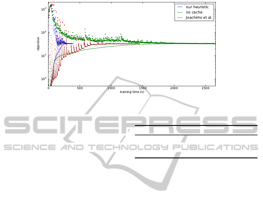
Figure 1: Training time comparison using different caching heuristics. Large dots correspond to o
Q
, small dots correspond to
o
C
, and the line shows o
W
. See the text for details.
4.3.2 Pascal VOC 2010
For the Pascal VOC 2010 dataset, we follow the pro-
cedure of Kr¨ahenb¨uhl and Koltun (2012) in using
the official “validation” set as our evaluation set, and
splitting the training set again. We use the unary po-
tentials provided by the same work, and compare only
against methods using the same setup and potentials,
Kr¨ahenb¨uhland Koltun (2013)and Dann et al. (2012).
Note that state-of-the-art approaches, some not build
on the CRF framework, obtain around a Jaccard In-
dex of 40% , notably Xia et al. (2012), who evaluate
on the Pascal VOC 2010 “test” set.
4.3.3 Results
We compare classification results using different in-
ference schemes in with results from the literature. As
a sanity check, we also provide results without pair-
wise interactions.
Results on the MSRC-21 dataset are shown in Ta-
ble 1. We find that our model is on par with state-of-
the-art approaches, implying that our model is realis-
tic for this task. In particular, our results are com-
parable to those of Lucchi et al. (2013), who use
a stochastic subgradient method with working sets.
Their best model takes 583s for training, while train-
ing our model exactly takes 1814s. We find it re-
markable that it is possible to guarantee optimality in
time of the same order of magnitude that a stochas-
tic subgradient procedure with approximate inference
takes. Using exact learning and inference does not
increase accuracy on this dataset. Learning the struc-
tured prediction model using move-making inference
alone takes 4 minutes, while guaranteeing optimality
up to ε = 10
−4
takes only 18 minutes.
Results on the Pascal-VOC dataset are shown in
Table 2. We compare against several approaches us-
Table 4: Objective function values on the Pascal Dataset.
Move-making Exact
Dual Objective o
W
92.06 92.24
Estimated Objective o
I
92.07 92.24
True Primal Objective o
E
92.35 92.24
ing the same unary potentials. For completeness, we
also list state-of-the-art approaches not based on CRF
models. Notably, our model matches or exceeds the
performance of the much more involved approaches
of Kr¨ahenb¨uhl and Koltun (2012) and Dann et al.
(2012) which use the same unary potentials. Using
exact learning and inference slightly increased per-
formance on this dataset. Learning took 25 minutes
using move-making alone and 100 minutes to guaran-
tee optimality up to ε = 10
−4
. A visual comparison of
selected cases is shown in Figure 2.
The objective function values using only the
under-generating move-making and the exact infer-
ence are detailed in Table 3 and Table 4. We see
that a significant gap between the cutting plane ob-
jective and the primal objective remains when using
only under-generating inference. Additionally, the es-
timated primal objectiveo
I
using under-generatingin-
ference is too optimistic, as can be expected. This un-
derlines the fact that under-generatingapproaches can
not be used to upper-bound the primal objective.
4.4 Implementation Details
We implemented the cutting plane Algorithm 1 and
our pairwise model in Python. Our cutting plane
solver for Equation (1) uses
cvxopt
(Dahl and Van-
denberghe, 2006) for solving the QP in the inner loop.
Code for our structured prediction framework will be
released under an open source license upon accep-
VISAPP2014-InternationalConferenceonComputerVisionTheoryandApplications
342
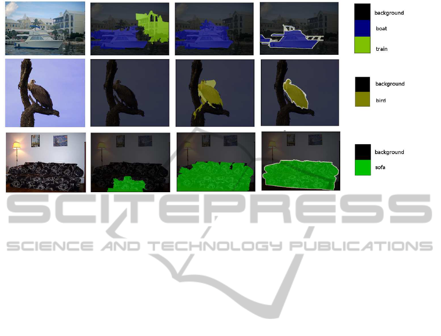
Figure 2: Visual comparison of the result of exact and approximate learning on selected images from the test set. From left to
right: the input image, prediction using approximate learning, prediction using exact learning, and ground truth.
tance.
We used the SLIC implementation provided by
Achanta et al. (2012) to extract superpixels and the
SIFT implementation in the
vlfeat
package (Vedaldi
and Fulkerson, 2008). For clustering visual words,
piecewise training of unary potentials and the ap-
proximation to the χ
2
-kernel, we made use of the
scikit-learn
machine learning package (Pedregosa
et al., 2011). The move-making algorithm using
QPBO is implemented with the help of the QPBO-
I method provided by Rother et al. (2007). We use
the excellent implementation of AD
3
provided by
the authors of Martins et al. (2011). Thanks to us-
ing these high-quality implementations, running the
whole pipeline for the pairwise model takes less than
an hour on a 12 core CPU. Solving the QP is done in
a single thread, while inference is parallelized over all
cores.
5 DISCUSSION
In this work we demonstrated that it is possible to
learn state-of-the-art CRF models exactly using struc-
tural support vector machines, despite the model con-
taining many loops. The key to efficient learning is
the combination of different inference mechanisms
and a novel caching scheme for the one-slack cutting
plane method, in combination with state-of-the-art in-
ference methods.
We show that guaranteeing exact results is feasi-
ble in a practical setting, and hope that this result pro-
vides a new perspective onto learning loopy models
for computer vision applications.
Even though exact learning does not necessarily
lead to a large improvement in accuracy, it frees the
practitioner from worrying about optimization and
approximation issues, leaving more room for improv-
ing the model, instead of the optimization.
We do not expect learning of pixel-level models,
which typically have tens or hundreds of thousands
of variables, to be efficient using exact inference.
However we believe our results will carry over to
other super-pixelbased approaches. Using other over-
generating techniques, such as duality-based message
passing algorithms, it might be possible to obtain
meaningful bounds on the true objective, even in the
pixel-level domain.
REFERENCES
Achanta, R., Shaji, A., Smith, K., Lucchi, A., Fua, P., and
S¨usstrunk, S. (2012). SLIC Superpixels Compared to
State-of-the-Art Superpixel Methods. Pattern Analy-
sis and Machine Intelligence.
Dahl, J. and Vandenberghe, L. (2006). Cvxopt: A python
package for convex optimization. In European Conv-
erence on Computer Vision.
Dann, C., Gehler, P., Roth, S., and Nowozin, S. (2012).
Pottics–the potts topic model for semantic image seg-
mentation. In German Conference on Pattern Recog-
nition (DAGM).
Everingham, M., Van Gool, L., Williams, C. K. I., Winn, J.,
and Zisserman, A. (2010). The Pascal Visual Object
Classes (VOC) Challenge. International Journal of
Computer Vision, 88.
Finley, T. and Joachims, T. (2008). Training structural
SVMs when exact inference is intractable. In Inter-
national Conference on Machine Learning.
LearningaLoopyModelExactly
343

Fulkerson, B., Vedaldi, A., and Soatto, S. (2009). Class
segmentation and object localization with superpixel
neighborhoods. In International Converence on Com-
puter Vision.
Gonfaus, J. M., Boix, X., van de Weijer, J., Bagdanov,
A. D., Serrat, J., and Gonzalez, J. (2010). Harmony
potentials for joint classification and segmentation. In
Computer Vision and Pattern Recognition.
Hazan, T. and Urtasun, R. (2010). A primal-dual message-
passing algorithm for approximated large scale struc-
tured prediction. In Neural Information Processing
Systems.
Joachims, T., Finley, T., and Yu, C.-N. J. (2009). Cutting-
plane training of structural SVMs. Machine Learning,
77(1).
Kohli, P., Torr, P. H., et al. (2009). Robust higher order po-
tentials for enforcing label consistency. International
Journal of Computer Vision, 82(3).
Komodakis, N. (2011). Efficient training for pairwise or
higher order crfs via dual decomposition. In Computer
Vision and Pattern Recognition.
Kr¨ahenb¨uhl, P. and Koltun, V. (2012). Efficient inference in
fully connected CRFs with Gaussian edge potentials.
Kr¨ahenb¨uhl, P. and Koltun, V. (2013). Parameter learning
and convergent inference for dense random fields. In
International Conference on Machine Learning.
Ladicky, L., Russell, C., Kohli, P., and Torr, P. H. (2009).
Associative hierarchical CRFs for object class image
segmentation. In International Converence on Com-
puter Vision.
Lempitsky, V., Rother, C., Roth, S., and Blake, A. (2010).
Fusion moves for markov random field optimization.
Pattern Analysis and Machine Intelligence, 32(8).
Lucchi, A., Li, Y., Boix, X., Smith, K., and Fua, P. (2011).
Are spatial and global constraints really necessary for
segmentation? In International Converence on Com-
puter Vision.
Lucchi, A., Li, Y., and Fua, P. (2013). Learning for struc-
tured prediction using approximate subgradient de-
scent with working sets. In Computer Vision and Pat-
tern Recognition.
Martins, A. F., Figueiredo, M. A., Aguiar, P. M., Smith,
N. A., and Xing, E. P. (2011). An augmented la-
grangian approach to constrained map inference. In
International Conference on Machine Learning.
Meshi, O., Sontag, D., Jaakkola, T., and Globerson, A.
(2010). Learning efficiently with approximate infer-
ence via dual losses. In International Conference on
Machine Learning.
Pedregosa, F., Varoquaux, G., Gramfort, A., Michel, V.,
Thirion, B., Grisel, O., Blondel, M., Prettenhofer, P.,
Weiss, R., Dubourg, V., et al. (2011). Scikit-learn:
Machine learning in python. Journal of Machine
Learning Research, 12.
Rother, C., Kolmogorov, V., Lempitsky, V., and Szummer,
M. (2007). Optimizing binary MRFs via extended
roof duality. In Computer Vision and Pattern Recog-
nition.
Shotton, J., Winn, J., Rother, C., and Criminisi, A. (2006).
Textonboost: Joint appearance, shape and context
modeling for multi-class object recognition and seg-
mentation. In European Converence on Computer Vi-
sion.
Szummer, M., Kohli, P., and Hoiem, D. (2008). Learning
CRFs using graph cuts. In European Converence on
Computer Vision.
Taskar, B., Guestrin, C., and Koller, D. (2003). Max-
margin markov networks. Neural Information Pro-
cessing Systems.
Tsochantaridis, I., Joachims, T., Hofmann, T., Altun, Y.,
and Singer, Y. (2006). Large margin methods for
structured and interdependent output variables. Jour-
nal of Machine Learning Research, 6(2).
Vedaldi, A. and Fulkerson, B. (2008). VLFeat: An open
and portable library of computer vision algorithms.
http://www.vlfeat.org/.
Vedaldi, A. and Zisserman, A. (2010). Efficient additive
kernels via explicit feature maps. In Computer Vision
and Pattern Recognition.
Xia, W., Song, Z., Feng, J., Cheong, L.-F., and Yan,
S. (2012). Segmentation over detection by coupled
global and local sparse representations. In European
Converence on Computer Vision.
VISAPP2014-InternationalConferenceonComputerVisionTheoryandApplications
344
