
Automatic Method for Sharp Feature Extraction from 3D Data of
Man-made Objects
Trung-Thien Tran, Van-Toan Cao, Van Tung Nguyen, Sarah Ali and Denis Laurendeau
Computer Vision and Systems Laboratory, Department of Electrical and Computer Engineering, Laval University, 1065,
Avenue de la M
´
edecine, G1V 0A6, Qu
´
ebec (QC), Canada
Keywords:
Sharp feature, Feature extraction, Projected distance, Point cloud and mesh processing.
Abstract:
A novel algorithm is proposed for extracting sharp features automatically from scanned 3D data of man-
made CAD-like objects. The input of our method consists of a mesh or an unstructured point cloud that is
captured on the object surface. First, the vector between a given point and the centroid of its neighborhood at
a given scale is projected on the normal vector and called the ’projected distance’ at this point. This projected
distance is calculated for every data point. In a second stage, Otsu’s method is applied to the histogram of
the projected distances in order to select the optimal threshold value, which is used to detect potential sharp
features at a single scale. These two stages are applied iteratively with the other incremental scales. Finally,
points recorded as potential features at every scale are marked as valid sharp features. The method has many
advantages over existing methods such as intrinsic simplicity, automatic selection of threshold value, accurate
and robust detection of sharp features on various objects. To demonstrate the robustness of the method, it is
applied on both synthetic and real 3D data of point clouds and meshes with different noise levels.
1 INTRODUCTION
Digital scanning devices have been used for various
applications. Due to the rapid development of scan-
ning technologies, large sets of accurate 3D points can
be collected with such devices. Therefore, more and
more applications use these sensors, especially in in-
dustrial manufacturing.
Among emerging problems, sharp feature extrac-
tion from scanned data of CAD model has recently
received much attention from the research commu-
nity. Sharp features help to understand the structure
of the underlying geometry of a surface. Futhermore,
it is very important on many issues such as segmenta-
tion (Lavou
´
e et al., 2005), surface reconstruction (We-
ber et al., 2012) and resampling (Huang et al., 2013).
Especially, most manufactured objects consist of the
combination of common geometric primitives such as
planes, cylinders, spheres, cones or toruses and the
intersection between these primitives can be consid-
ered as sharp features. The input 3D data consists
of meshes or point clouds. Therefore, existing meth-
ods are classified into two categories: mesh-based and
point-based methods. Most existing methods focus
only on point clouds or meshes which limits their flex-
ibility and generality.
Several techniques (Hubeli and Gross, 2001;
Ohtake et al., 2004; Hildebrandt et al., 2005) use
polygonal meshes as input. In (Hubeli and Gross,
2001), a framework to extract mesh features from sur-
faces is presented. However, this approach is semi-
automatic, that is the user is required to input a few
control parameters before a solution is found. Hilde-
brandt et al. (Hildebrandt et al., 2005) have also pro-
posed a new scheme based on discrete differential ge-
ometry, avoiding costly computations of higher order
approximating surfaces. This scheme is augmented
by a filtering method for higher order surface deriva-
tives to improve both the stability and the smooth-
ness of feature lines. Ohtake et al. (Ohtake et al.,
2004) propose to use an implicit surface fitting proce-
dure for detecting view and scale independent ridge-
valley structures on triangle meshes. Nevertheless,
the methods still require thresholding value for scale-
independent parameter in order to keep the most visu-
ally important features. Moreover, the methods only
show the results of feature lines for graphics models.
Point cloud preserves the structure of the underly-
ing surface, so it recently has been used in process-
ing and modelling. Sharp features are normally found
at the points that have large variation in curvature or
discontinuities in normal orientation of the surface.
112
Tran T., Cao V., Nguyen V., Ali S. and Laurendeau D..
Automatic Method for Sharp Feature Extraction from 3D Data of Man-made Objects.
DOI: 10.5220/0004674801120119
In Proceedings of the 9th International Conference on Computer Graphics Theory and Applications (GRAPP-2014), pages 112-119
ISBN: 978-989-758-002-4
Copyright
c
2014 SCITEPRESS (Science and Technology Publications, Lda.)

Consequently, several approaches (Demarsin et al.,
2007) detect sharp features using differential geom-
etry principles exploiting surface normal and curva-
ture information. Nevertheless, the first step of this
method is a normal-based segmentation that does not
guarantee the quality of results because of noisy point
data. Merigot et al. (M
´
erigot et al., 2011) compute
principal curvatures and normal directions of the un-
derlying surface through Voronoi covariance measure
(VCM). Then they estimate the location and direction
of sharp features using Eigen decomposition. How-
ever, this method requires significant computational
time for calculating the VCM.
Recently, Gumhold et al. (Gumhold et al., 2001)
use PCA to calculate the penalty function that takes
into consideration curvature, normal and correlation.
Pauly et al. (Pauly et al., 2003) calculate surface vari-
ation using the same mathematical technique. Weber
et al. (Weber et al., 2010) have proposed to use sta-
tistical methods to infer local surface structure based
on Gaussian map clustering. Park et al. (Park et al.,
2012) used tensor voting to infer the structure near a
point. However, all these methods require that many
parameters be set manually.
This paper proposes a novel algorithm for extract-
ing sharp features automatically from 3D data, which
is developed from our previous work (Tran et al.,
2013). We first preprocess the scanned data by find-
ing the neighborhood and estimating the surface nor-
mal at each point. The main contribution of this pa-
per is the use of the projected distance calculated in
a neighborhood. Then an automatic threshold value
is selected by Otsu’s method to detect potential sharp
features at a given scale. The process is iteratively ap-
plied for incremental scales. In the end, valid sharp
features are determined by multi-scale analysis as a
refinement. Generally, our method focuses on two
main computation steps: (i) calculating the projected
distance at a single scale and automatically extracting
potential sharp features. (ii) applying these calcula-
tions at multiple scales. Therefore, the strong points
of the proposed method are summarized in the follow-
ing:
• The proposed method is very simple and fast. Fur-
thermore, the method accepts both meshes and
unstructured point clouds as input. This allows
the method to work without conversion between
types of data and adds flexibility to the technique.
• No parameter needs to be set by the user since the
entire process is completely automatic. This is a
significant advantage over existing methods.
• Our approach explores multiple scales in order to
extract sharp features accurately with certain lev-
els of noise. In most cases, the detected features
are one-point wide.
• Accurate and robust results are achieved by the
method even for noisy data and complex object
geometry.
The rest of this paper is organized as follows.
Neighborhood and normal estimation for meshes and
point clouds are described in Section 2. The proposed
algorithm is described in Section 3. Results and dis-
cussion are presented in Section 4, while Section 5
draws some conclusions on the proposed method.
2 POINT NEIGBORHOOD AND
SURFACE NORMAL
ESTIMATION
The input 3D data can consist of meshes or point
clouds that have different structures to represent the
underlying surface of a given object. The neigh-
borhood around a point is used to estimate the nor-
mal at that point. Therefore, the problem of finding
the neighborhood of each point is addressed first and
the problem of estimating the normal vector for each
point is then described according to the type of data.
2.1 Point Clouds
A point cloud is defined as a set of points within a
three-dimensional coordinate system. This type of
data acquired from the scanners represents noisy sam-
ples of the object surface. The information about con-
nectivity and surface normal of underlying surfaces is
lost completely in the sampling process. Moreover, it
resides implicitly in the relationship between a sam-
pled point and its neighborhood. Hence, the first step
in surface normal estimation at a given point is to find
the number of points around this point. In this paper,
the data is structured by using k-d trees (Weiss, 1994)
to search the k nearest neighborhood.
Classical principal component analysis PCA in
(Hoppe et al., 1992) is usually selected for normal
estimation because of its simplicity and efficiency.
However, a point cloud contains a set of non-uniform
points, so a weight that is derived from the distance
to the centroid should be assigned to each point in
the neighborhood in order to improve the robustness
of the method. A covariance matrix CV of point p
i
is established in Equation (1) and analyzed and the
eigenvector corresponding to the smallest eigenvalue
is considered as the normal vector n
i
at point p
i
.
CV
i
=
∑
j∈N(i)
µ
j
(p
j
− p
i
)
T
(p
j
− p
i
) ∈ R
3×3
(1)
AutomaticMethodforSharpFeatureExtractionfrom3DDataofMan-madeObjects
113
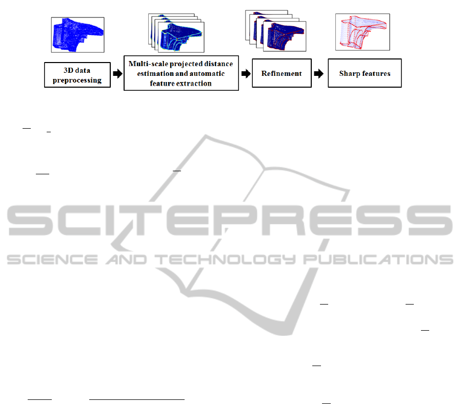
Figure 1: Overall procedure of the proposed method.
where
p
i
=
1
k
∑
j∈N(i)
p
j
is p
i
’s local data centroid,
N(i) is the set of k points in the neighborhood around
point p
i
. µ
j
is calculated by the Gaussian function
µ
j
= exp(
−d
2
j
k
2
) of the distance d
j
= kp
j
− p
i
k. The
scale k is the number of neighboring points.
2.2 Meshes
A polygonal mesh is a collection of vertices, edges
and faces that represents the shape of a object. This
type of data is different from point clouds because it
contains edges connecting the vertices. Therefore, an
approach is needed to find the neighborhood of a point
based on this connection. A k-ring neighborhood of
a vertex p
i
is defined as a set of vertices that are con-
nected to p
i
by at most k edges.
A simple and effective method for normal vector
estimation is to calculate it as the weighted average of
the normal vectors of the triangles formed by p
i
and
pairs of its neighbours inside the 1-ring. The basic
averaging method is based on Equation (2):
n
i
=
1
|N(i)|
∑
j∈N(i)
ω
j
[p
j
− p
i
] × [p
j+1
− p
i
]
|[p
j
− p
i
] × [p
j+1
− p
i
]|
(2)
where p
j
is one of the points inside 1-ring. ω
j
is a normalized weighting factor that can be calcu-
lated by angle-weighted, area-weighted and centroid-
weighted methods. A good summary of these meth-
ods can be found in (Jin et al., 2005). In this paper, we
use a simple method proposed by Gouraud (Gouraud,
1971) (ω
j
= 1).
3 PROPOSED METHOD FOR
EXTRACTING SHARP
FEATURES
In this section, we describe our algorithm for extract-
ing sharp features at multiple scales. A block dia-
gram of the method is shown in Figure 1. First, the
projected distance definition and the calculation pro-
cedure for each point are introduced in Section 3.1.
Then a threshold value is seclected automatically by
Otsu’s algorithm in Section 3.2. After this step, poten-
tial sharp features are detected at a given scale. These
steps are applied iteratively for multiple scales. The
approach for detecting valid and reliable sharp fea-
tures is described in Section 3.3.
3.1 Projected Distance Calculation
The projected distance is a value calculated by pro-
jecting the vector between a given point and the cen-
troid of its neighborhood at a given scale on the nor-
mal as given in Equation (3). The procedure is shown
in Figure 2.
pdis(i) = abs(
−−−−−→
(p
i
−
p
i
)·
−→
n
i
) = abs(k
−−−−→
p
i
− p
i
k·cos θ
i
)
(3)
where θ
i
is the angle between vector
−−−−−→
(p
i
− p
i
) and
vector
−→
n
i
, which is the surface normal at point p
i
cal-
culated in Section 2.1 or Section 2.2 according to the
type of input data. p
i
is the centroid of neighborhood
points determined with the k-d tree for point clouds
Section 2.1 or k-ring for meshes Section 2.2. Angle θ
i
between vector
−−−−−→
(p
i
− p
i
) and vector
−→
n
i
can be greater
or smaller than 90 degrees, but the projected distance
is always a positive number. That is why the direction
of the normal vector is not considered here as it is in
(Hoppe et al., 1992), only the orientation is used in
our work.
The projected distance value expresses the struc-
ture of the underlying surface supported by the neigh-
borhood. Therefore, the central idea of our method is
that the projected distance is almost zero for a point
lying on a smooth surface area. However, the pro-
jected distance has a large value if a point is located
on or near a sharp feature, as shown in Figure 3. Our
method uses this property of the projected distance to
assess whether a point is located on a sharp feature or
not.
GRAPP2014-InternationalConferenceonComputerGraphicsTheoryandApplications
114
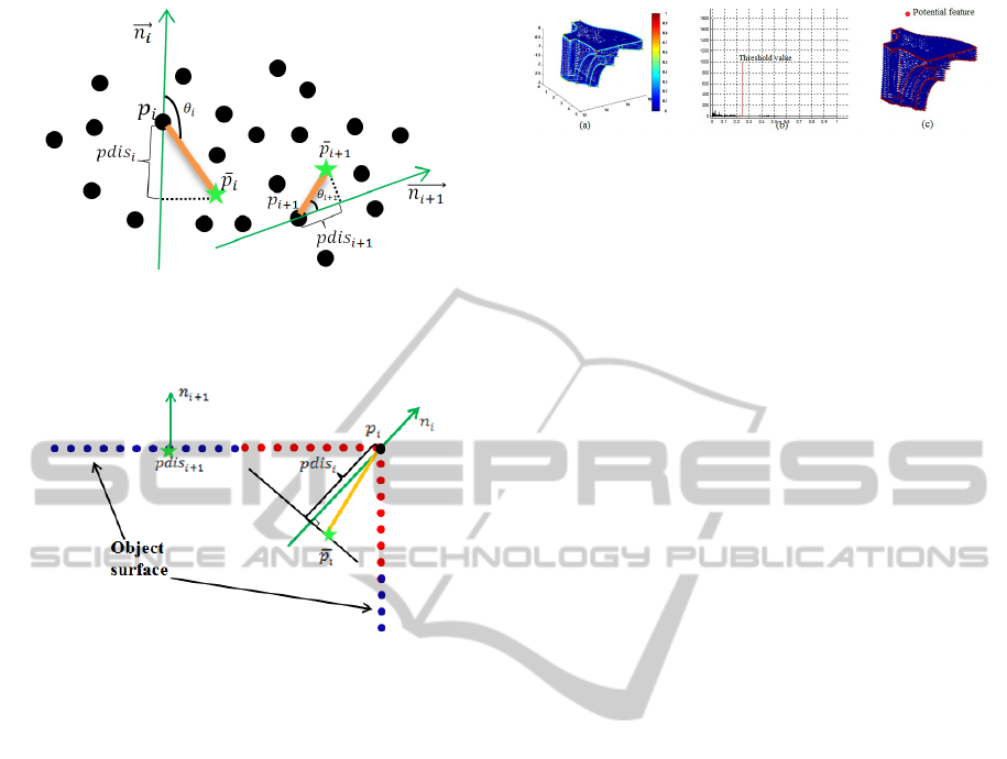
Figure 2: Procedure for calculating the projected distance
at each point. The green star is the centroid of the neighbor-
hood.
Figure 3: Projected distances calculated at smooth (blue
points) and sharp areas (red points). Green points are the
centroids of the data.
3.2 Automatic Selection of a Threshold
Value for the Detection of Sharp
Features
The projected distances for every data point (point
cloud or mesh) was computed at the same scale in
the previous section. Potential sharp features are de-
tected at a given scale. First, every projected distance
is normalized between [0,1] as displayed in Figure
4(a). Then a threshold value for the projected dis-
tance needs to be calculated to evaluate whether or
not a given point is located on a sharp feature. Otsu’s
method (Otsu, 1979) is a optimal method for this non-
trivial task and was chosen because of its simplicity
and efficiency. Furthermore, it contributes in mak-
ing our method completely automatic. The input to
Ostu’s method being a histogram, a histogram of the
normalized projected distance values is generated and
shown in Figure 4(b).
Otsu’s algorithm is based on the very simple idea
of finding the threshold value that minimizes the
weighted within-class variance. This turns out to be
the same as maximizing the between-class variance.
Threshold T allows the generation of a binary version
Figure 4: Automatic threshold estimation and feature ex-
traction. (a) Normalized projected distance. (b) Histogram
and threshold value. (c) Sharp feature candidates.
of projected distance values by setting all vertices be-
low the threshold to zero and all vertices above that
threshold to one Equation (4).
f (i) =
1 if pdis(i) ≥ T
0 if pdis(i) < T
(4)
where f (i) is a binary version of pdis(i) with global
threshold T at the red line in Figure 4(b). The points
for which f (i) is equal to one are considered as po-
tential sharp features. Potential sharp features are ex-
tracted by Equation (4) and displayed in Figure 4(c).
3.3 Multiscale Processing and
Refinement
Potential sharp features are extracted from the steps
decribed in the two previous sections at a single scale.
A real feature can be recognized at multiple scales by
a human. Besides, the result at a single scale may
contain several false feature points because of noise.
Therefore, the proposed method calculates the pro-
jected distance and extracts sharp features automati-
cally at multiple scales to eliminate false sharp fea-
tures.
Valid sharp features are those recorded at all
scales. Hence, Equation (5) explains the means of
deciding whether or not a point is valid sharp feature:
F(i) =
1 if
∑
ns
i=1
f (i) = ns
0 if
∑
ns
i=1
f (i) < ns
(5)
where F(i) is the final sharp feature map, ns is the
number of scales that are investigated for point clouds
or meshes in Section 4.2 and f (i) is calculated from
Equation (4) in Section 3.2. The results of the mul-
tiscale sharp feature extraction method are shown in
Figure 9 and Figure 10 for point clouds and meshes,
respectively.
4 RESULTS AND DISCUSSION
We have tested the proposed method on various com-
plex models corrupted by different noise levels. Fur-
thermore, the results provided by our method are
AutomaticMethodforSharpFeatureExtractionfrom3DDataofMan-madeObjects
115
compared with some other methods using mean cur-
vature (Yang and Lee, 1999; Watanabe and Belyaev,
2001), normal vector (Hubeli and Gross, 2001) and
surface variation in Pauly’s method (Pauly et al.,
2003) for point-based methods and Ohtake’s method
(Ohtake et al., 2004) for mesh-based methods. Com-
putation time and limitations of our method are also
reported.
4.1 Comparison with Other Methods
4.1.1 Point-based Method
As mentioned above, a sharp feature is a point at
which the surface normal vector (Demarsin et al.,
2007) or the curvature (Yang and Lee, 1999) is dis-
continuous in value, so the Mean curvature and the
normal difference between adjacent triangles are used
as the factors for determining sharp feature locations.
It assigns a value w
i
defined by normal difference be-
tween given point and its neighborhood (Hubeli and
Gross, 2001).
w
i
=
1
|N(i)|
∑
j∈N(i)
cos(
n(i)
kn(i)k
.
n( j)
kn( j)k
)
−1
(6)
where n(i), n( j) and N(i) are defined in Section 2.1.
In (Pauly et al., 2003), Pauly et al. use surface
variation σ
i
, which is calculated as the ratio between
the smallest eigenvalue and sum of the eigenvalues of
the covariance matrix CV
i
in Equation 1 established
by the neighborhood around a given point.
σ
i
=
λ
0
λ
0
+ λ
1
+ λ
2
(7)
Therefore, we will compare our method based on
the projected distance with these three parameters.
We investigate these methods by applying them to the
fandisk point cloud at a single scale (k=16), that was
mentioned as the optimal one in (Weber et al., 2010).
Moreover, the other three methods are not automatic
and require some threshold values to be set, so our au-
tomatic threshold estimation is applied to them. The
results of the four methods are shown in Figure 5 and
Figure 6.
Figure 5: Sharp feature extraction using different parame-
ters for the fandisk model. (a) Normal. (b) Mean curvature.
(c) Surface variation (Pauly et al., 2003). (d) Projected dis-
tance.
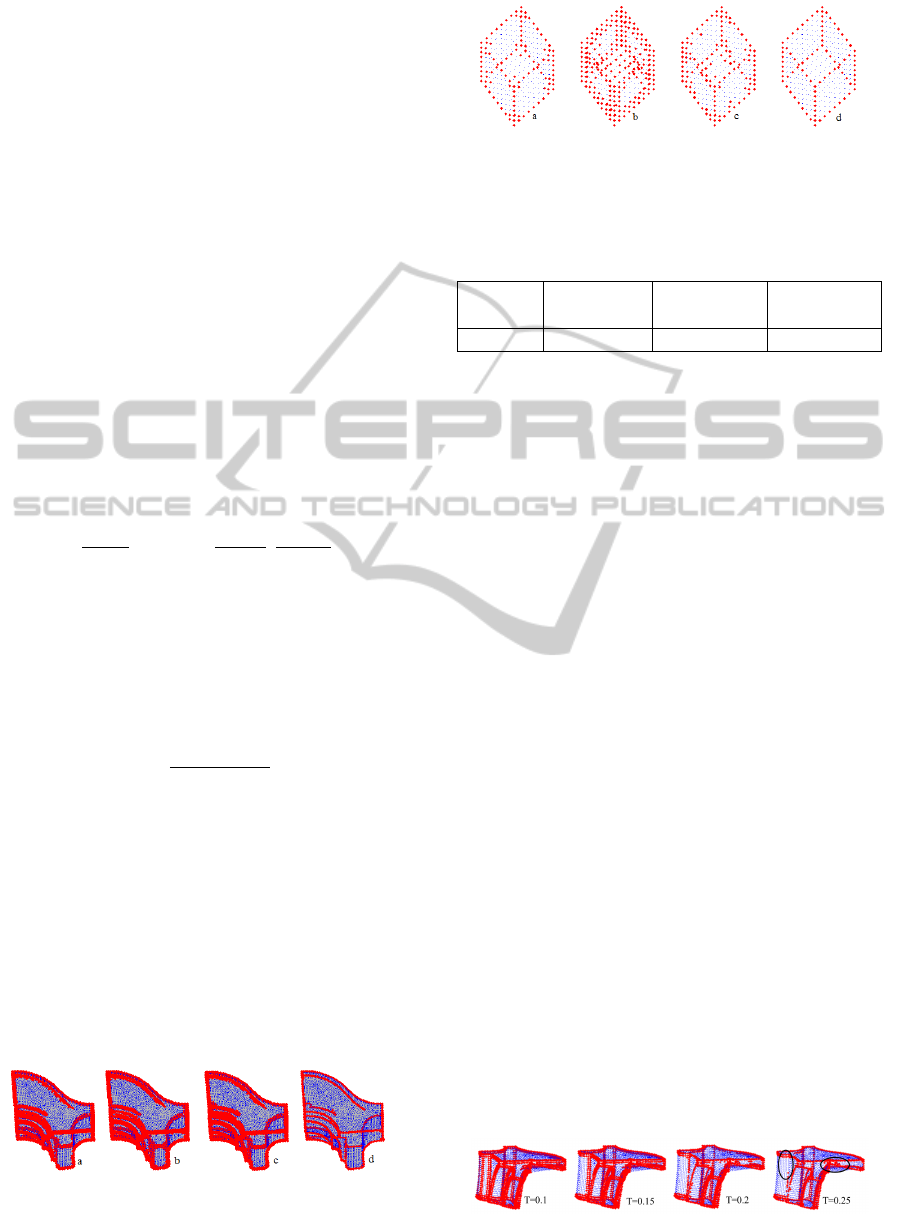
Figure 6: Sharp feature extraction using different parame-
ters for synthetic cube model. (a) Normal. (b) Mean curva-
ture. (c) Surface variation (Pauly et al., 2003). (d) Projected
distance.
Table 1: Number of detected sharp features on the cube
model by 4 methods.
Normal Mean cur-
vature
Surface
variation
Projected
distance
116 248 135 91
Observing Figure 5 and Figure 6 indicates that
our method is able to detect sharp features that are
one point wide. Mean curvature, normal and Pauly’s
methods detect rather thick features including many
potential feature points. Because the mean curvature
and the surface normal do not reveal shape informa-
tion of the underlying surface as the projected dis-
tance does. The projected distance is small at smooth
and near-edge points and much smaller than the value
at sharp features. Therefore, the feature lines detected
by the proposed method are thinner and more accu-
rately located. The results prove that ’projected dis-
tance’ is a better factor that can be used for detecting
sharp features.
Figure 7 shows that even when tuning the thresh-
old value manually to improve its performance,
Pauly’s method still fails to produce thin and accu-
rate features. For instance on threshold values for sur-
face variation set at T=0.1, 0.15 and 0.2, the results
contain many spurious sharp features. With threshold
T=0.25, some good features are missing and the result
still contains spurious sharp features (black ellipse in
Figure 7).
Futhermore, the absolute accuracy of our method
is demonstrated in Figure 6 and Table 1. A synthetic
cube point cloud was generated with 91 sharp features
composed of 386 data points. Mean curvature, normal
and Pauly’s method detect many spurious sharp fea-
tures while our method extracts all 91 sharp features
correctly and at the right location.
Figure 7: Sharp features extracted with tuning threshold for
Pauly’s method.
GRAPP2014-InternationalConferenceonComputerGraphicsTheoryandApplications
116
4.1.2 Mesh-based Method
In this section, we compare the results of the mesh-
based method to Ohtake’s method (Ohtake et al.,
2004). His method uses an implicit surface fitting
procedure for detecting ridge-valley structure on sur-
face approximated by dense triangulation. His im-
plemented code is available from the author’s website
and the selected threshold settings are the default val-
ues for scale-independent parameter, connecting and
iterations. The results are shown in Figure 8. In his
results, ridge and valley points are displayed in red
and blue, respectively. We find that valley points are
located on smooth areas while ridge points are miss-
ing at sharp features such as at the edge of the block
model. On the other hand, our method obtains the
sharp features accurately and does not include valley
points (blue) as in his method. Moreover, his method
detects many spurious sharp features at the small and
thin holes as shown in Figure 8.
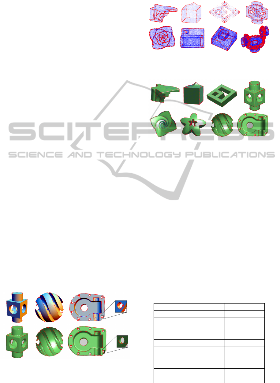
4.2 Results for Various Models
The method is applied on other meshes and
point clouds. Most models are taken from the
AIM@SHAPE Shape Repository and the Octa-flower
model from Ohtake. With point cloud models, we in-
vestigated the behaviour of the proposed method at
multiple scales k= (12,16,...40) and Figure 9 shows
the results for several point cloud models. Although
these models contain many different primitives in-
cluding planes, spheres, cylinders and even free-form
primitives, our method can detect sharp features ac-
curately in each model. For meshes, 1,2,3 and 4-
ring neighborhoods are used to calculate the projected
distances for every vertex. Figure 10 shows the re-
sults for some mesh models and demonstrates the ef-
ficiency of the method to detect thin sharp features.
Figure 8: Sharp features extracted from Block, Sharp-
feature and Casting models using Ohtake’s method (Ohtake
et al., 2004) (upper row) and our mesh-based method (lower
row).
Figure 9: Sharp features extracted from point clouds: Fan-
disk, Smooth-feature, Double-torus2, Block, Octa-flower,
Cylinder, Box, BEVEL2, respectively.
Figure 10: Sharp features extracted from meshes: Fandisk,
Smooth-feature, Double-torus2, Block, Octa-flower, Trim-
star, Sharp-sphere, Casting, respectively.
4.3 Computation Cost
The proposed method are executed on Matlab on a 3.2
GHz Intel Core i7 platform. Table 2 for point clouds
and Table 3 for meshes show the computation time of
the method. This process is implemented without par-
allel processing. We believe that a C++ implementa-
tion would speed up the process significantly and par-
allel processing could be applied to process multiple
scales simultaneously.
4.4 Robustness to Noise
To illustrate the robustness of the proposed method to
a certain level of noise, some results for noisy fan-
Table 2: Timing of our proposed method for point cloud
models.
Model name Points Total time (s)
Fandisk 6475 1.05
Smooth-feature 6177 1.01
Double-torus2 2668 0.44
Block 12909 2.01
Octa-flower 12868 2.11
Cylinder 50000 8.34
Box 50000 8.21
BEVEL2 64250 4.92
Real data1 108349 17.4
Real data2 30751 4.99
AutomaticMethodforSharpFeatureExtractionfrom3DDataofMan-madeObjects
117
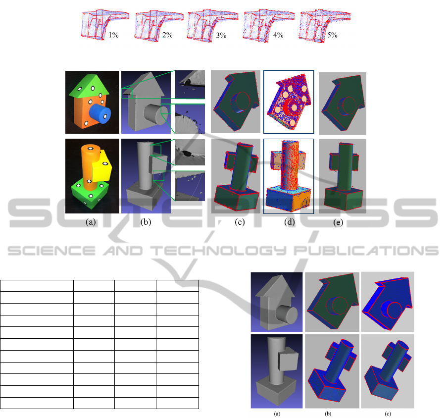
Figure 11: Sharp features extracted from fandisk model with different levels of noise.
Figure 12: Results on noisy data with outliers and holes: (a) Original object and markers. (b) Scanned data with outliers and
holes. (c) Pauly’s method (Pauly et al., 2003). (d) Ohtake’s method (Ohtake et al., 2004). (e) Our Method.
Table 3: Timing of our proposed method for mesh models.
Model name Points Faces Time(s)
Fandisk 6475 12946 1.48
Smooth-feature 6177 12350 1.40
Double-torus2 2668 5340 0.61
Block 2132 4272 0.52
Octa-flower 7919 15834 1.79
Trim-star 5192 10384 1.18
Sharp-sphere 8271 16538 1.87
Casting 5086 10204 0.42
Real data1 108349 214189 21.4
Real data2 30751 60783 6.84
disk point cloud models and real data are presented in
this section. First, Gaussian noise with zero mean and
standard deviations of 1-5 % of the average distance
between points was added to the point cloud data.
Then our method is applied to this data corrupted by
noise. Figure 11 shows the results for different noise
levels. For a noise level of (1-3)% acceptable results
are still achieved. For a noise level of (4-5)% a small
part of the model is contaminated by spurious feature
points. Therefore, applying a prior denoising algo-
rithm could help the proposed method to obtain better
results.
Figure 12 shows the results on real scanned
data, which contains many outliers and holes Figure
12(b). The data is captured by the GO! scan sensor
(http://www.goscan3d.com). Other methods such as
Pauly’s (Figure 12(c)) and Ohtake’s (Figure 12(d))
Figure 13: Results on preprocessed real data: (a) Smoothed
and hole-filled data. (b) Point-based method. (c) Mesh-
based method.
methods are also tested. Observing the results indi-
cates that Pauly’s method misses several sharp fea-
tures, while Ohtake’s method fails totally for noisy
data.
4.5 Limitations
Although the proposed method can extract sharp fea-
tures accurately, it also depends on the level of noise
of the captured data and also on the distribution of the
data. For instance for areas with low density, the im-
provement brought by the weighting factor is minor.
Therefore, preprocessing stages such as resampling
GRAPP2014-InternationalConferenceonComputerGraphicsTheoryandApplications
118

and pre-filtering would be necessary in these cases to
improve the results. Figure 13 shows the results af-
ter removing outliers and filling holes in real scanned
data, sharp features are detected accurately.
5 CONCLUSIONS
We have introduced an automatic method for extract-
ing sharp features from 3D data. This method accepts
both meshes and point clouds as input. The projected
distance is calculated at multiple scales, which is sup-
ported by the k neareast neighborhood in point clouds
or the k-ring neighborhood in meshes. Then reliable
sharp features are extracted automatically by using
Otsu’s method. In addition to its simplicity, the pro-
posed method outperforms other methods presented
in the literature.
In the future, the algorithm could be improved by
connecting discrete sharp features into parametrized
curves for obtaining high-level descriptions. Further-
more, we plan to use the results of our algorithm for
practical problems such as remeshing or mesh gener-
ation.
ACKNOWLEDGEMENTS
The authors thank the AIM@SHAPE Shape Reposi-
tory and Ohtake for making their codes and models
available. This research project was supported by the
NSERC/ Creaform Industrial Research Chair on 3-D
Scanning.
REFERENCES
Demarsin, K., Vanderstraeten, D., Volodine, T., and Roose,
D. (2007). Detection of closed sharp edges in point
clouds using normal estimation and graph theory.
Comput. Aided Des., 39(4):276–283.
Gouraud, H. (1971). Continuous shading of curved sur-
faces. IEEE Trans. Comput., 20(6):623–629.
Gumhold, S., Wang, X., and Macleod, R. (2001). Feature
extraction from point clouds. In In Proceedings of the
10 th International Meshing Roundtable, pages 293–
305.
Hildebrandt, K., Polthier, K., and Wardetzky, M. (2005).
Smooth feature lines on surface meshes. In Proceed-
ings of the third Eurographics symposium on Geom-
etry processing, SGP ’05, Aire-la-Ville, Switzerland,
Switzerland. Eurographics Association.
Hoppe, H., DeRose, T., Duchamp, T., McDonald, J., and
Stuetzle, W. (1992). Surface reconstruction from un-
organized points. In Proceedings of the 19th an-
nual conference on Computer graphics and interac-
tive techniques, SIGGRAPH ’92, pages 71–78, New
York, NY, USA. ACM.
Huang, H., Wu, S., Gong, M., Cohen-Or, D., Ascher, U.,
and Zhang, H. R. (2013). Edge-aware point set re-
sampling. ACM Trans. Graph., 32(1):9:1–9:12.
Hubeli, A. and Gross, M. (2001). Multiresolution feature
extraction for unstructured meshes. In Proceedings
of the conference on Visualization ’01, VIS ’01, pages
287–294, Washington, DC, USA. IEEE Computer So-
ciety.
Jin, S., Lewis, R. R., and West, D. (2005). A comparison of
algorithms for vertex normal computation. The Visual
Computer, 21(1-2):71–82.
Lavou
´
e, G., Dupont, F., and Baskurt, A. (2005). A new cad
mesh segmentation method, based on curvature tensor
analysis. Comput. Aided Des., 37(10):975–987.
M
´
erigot, Q., Ovsjanikov, M., and Guibas, L. (2011).
Voronoi-based curvature and feature estimation from
point clouds. Visualization and Computer Graphics,
IEEE Transactions on, 17(6):743–756.
Ohtake, Y., Belyaev, A., and Seidel, H.-P. (2004). Ridge-
valley lines on meshes via implicit surface fitting.
ACM Trans. Graph., 23(3):609–612.
Otsu, N. (1979). A threshold selection method from gray-
level histograms. IEEE Transactions on Systems, Man
and Cybernetics, 9(1):62–66.
Park, M. K., Lee, S. J., and Lee, K. H. (2012). Multi-scale
tensor voting for feature extraction from unstructured
point clouds. Graph. Models, 74(4):197–208.
Pauly, M., Keiser, R., and Gross, M. (2003). Multi-scale
feature extraction on point-sampled surfaces. Com-
puter Graphics Forum, 22(3):281–289.
Tran, T. T., Ali, S., and Laurendeau, D. (2013). Automatic
sharp feature extraction from point clouds with opti-
mal neighborhood size. In The Thirteenth IAPR Inter-
national Conference on Machine Vision Applications,
MVA ’13, pages 165–168, Kyoto, Japan.
Watanabe, K. and Belyaev, A. G. (2001). Detection of
salient curvature features on polygonal surfaces. Com-
puter Graphics Forum, 20(3):385–392.
Weber, C., Hahmann, S., and Hagen, H. (2010). Sharp fea-
ture detection in point clouds. In Proceedings of the
2010 Shape Modeling International Conference, SMI
’10, pages 175–186, Washington, DC, USA. IEEE
Computer Society.
Weber, C., Hahmann, S., Hagen, H., and Bonneau, G.-P.
(2012). Sharp feature preserving mls surface recon-
struction based on local feature line approximations.
Graph. Models, 74(6):335–345.
Weiss, M. A. (1994). Data structures and algorithm analy-
sis (2. ed.). Benjamin/Cummings.
Yang, M. and Lee, E. (1999). Segmentation of measured
point data using a parametric quadric surface approx-
imation. Computer-Aided Design, 31(7):449 – 457.
AutomaticMethodforSharpFeatureExtractionfrom3DDataofMan-madeObjects
119
