Active Contour Segmentation with Afﬁne Coordinate-based

Parametrization

Q. Xue

1,2

, L. Igual

, A. Berenguel

, M. Guerrieri

and L. Garrido

Departament de Matem

atica Aplicada i An

alisi, Universitat de Barcelona, Barcelona, Spain

Department of Mathematics, Tongji University, Shanghai, China

Departament d’Inform

atica i Matem

atica Aplicada, Universitat de Girona, Girona, Spain

Keywords:

Active Contours, Afﬁne Coordinates, Mean Value Coordinates.

Abstract:

In this paper, we present a new framework for image segmentation based on parametrized active contours. The

contour and the points of the image space are parametrized using a set of reduced control points that have to

form a closed polygon in two dimensional problems and a closed surface in three dimensional problems. By

moving the control points, the active contour evolves. We use mean value coordinates as the parametrization

tool for the interface, which allows to parametrize any point of the space, inside or outside the closed polygon

or surface. Region-based energies such as the one proposed by Chan and Vese can be easily implemented in

both two and three dimensional segmentation problems. We show the usefulness of our approach with several

experiments.

1 INTRODUCTION

Active contours have been proved to be a powerful

tool for segmentation in image processing. In ac-

tive contours an evolving interface is propagated in

order to recover the shape of the object of interest.

In a two dimensional problem, the evolving interface

is a contour whereas in a three dimensional prob-

lem the evolving interface is a surface. The inter-

face is evolved by minimizing an energy that math-

ematically expresses the properties of the object to

be segmented. In this energy functional, the terms

corresponding to image features can be either edge-

based and/or region-based. Edge-based terms mea-

sure features on the evolving interface to identify ob-

ject boundaries and are usually based on a function

of the image gradient (Caselles et al., 1997). They are

known to be sensitive to noise and thus energies based

on such type of features usually need the evolving in-

terface to be initialized near the solution.

Region-based terms were introduced by Chan and

Vese (Chan and Vese, 2001). In this case some fea-

tures that are measured inside and outside of the re-

gions allows to evolve the interface and thus drive

the energy to its minimum. Chan and Vese mini-

mize the variance of the gray-level in the interior and

exterior regions. Region-based terms are known to

be more robust to noise than edge-based terms and

thus they usually do not need the initialization to be

near the solution. Since the work of Chan and Vese

other approaches have extended the idea by measur-

ing other types of features (Rousson and Deriche,

2002; Michailovich et al., 2007). However, the lat-

ter approaches do measure the features in the whole

inner and outer regions and thus may fail if these fea-

tures are not spatially invariant. This problem has

been tackled in (Lankton and Tannenbaum, 2008),

in which the inner and outer regions are deﬁned by

means of a band around the evolving interface. Thus,

their approach is suited for segmenting objects having

heterogeneous properties.

Depending on the representation of the evolving

interface, active contours may be classiﬁed into para-

metric or geometric ones. In parametric approaches

the interface in two dimensional problems may be de-

scribed by means of a set of discrete points (Kass

et al., 1988) or using basis functions such as B-

splines (Jacob et al., 2004). In three dimensional

problems, parametrizations using B-Splines (Barbosa

et al., 2012) have also been used. In general, using

basis functions such as B-splines allows to use less

parameters to represent the curve than directly dis-

cretizing the curve or surface and have inherent regu-

larity and hence do not require additional constraints

to ensure smoothness. Parametric contours are able

to deal easily with edge-based energies. However,

Xue Q., Igual L., Berenguel A., Guerrieri M. and Garrido L..

Active Contour Segmentation with Afﬁne Coordinate-based Parametrization.

DOI: 10.5220/0004677200050014

In Proceedings of the 9th International Conference on Computer Vision Theory and Applications (VISAPP-2014), pages 5-14

ISBN: 978-989-758-003-1

 2014 SCITEPRESS (Science and Technology Publications, Lda.)

dealing with region-based energies is more difﬁcult,

see (Jacob et al., 2004; Barbosa et al., 2012) for in-

stance. Moreover, parametric approaches require the

user to deﬁne the number of control points that will

be used to evolve the contour and it is difﬁcult to deal

with topological changes. This has favored that many

works have been tackled using geometric approaches.

Geometric approaches represent the evolving in-

terface as the zero level set of a higher dimensional

function, which is usually called level set function.

Therefore geometric approaches are also called level

set approaches. Level set approaches are able to cope

with the change of the curve topology and thus are

able to segment multiple unconnected regions. This

property has made level sets very popular approaches.

However, level set approaches are usually computa-

tionally more complex and difﬁcult to deal with since

they increase the dimension of the problem by one.

This makes level sets a difﬁcult approaches in three-

dimensional applications which are common in med-

ical image segmentation.

In this paper, we focus on parametric representa-

tions due to its computational advantages and simplic-

ity. A direct consequence of the explicit formulation

is the loss of topological ﬂexibility. However, this

limitation is a mild constraint in many applications,

where the goal may be to simply segment one con-

nected object and thus the topological ﬂexibility of

the level sets is not needed.

We contribute with a novel framework for seg-

menting two and three dimensional connected ob-

jects using a new class of parametric active contours.

The parametrization is based on a class of deformable

models well known in computer graphics such as the

animation of characters for video games or movies.

Such models are usually made up of millions of tri-

angles. The motion of the character is controlled by

a reduced number of control points: when these con-

trol points move the associated character deforms ac-

cordingly. A similar idea is applied in our paper: the

evolving interface, the interior and exterior regions

are parametrized by a set of control points. When

these control points move the interface evolves cor-

respondingly to the object to be segmented.

Our work stems from the ideas of free-form de-

formations (Faloutsos et al., 1997; Coquillart, 1990).

Free-form deformations have been actively used for

medical image registration (Rueckert et al., 1999).

However, to the best of our knowledge, free-form de-

formations have not been used for parametric active

contours. In our work we use the mean value co-

ordinates as the parametrization tool for the evolv-

ing interface (Floater, 2003). Mean value coordinates

have several advantages over free-form deformation,

namely that control points only need to form a closed

polygon in two dimensional problems (or surface in

three dimensional problems) that may have any shape.

Any point of the space, inside or outside of this poly-

gon (or surface), can be parametrized with respect to

the control points. For free-form deformations the

control points need to form a regular shape and only

interior points can be parametrized.

The rest of the paper is organized as follows: Sec-

tion 2 reviews the related state-of-the-art work. Sec-

tion 3 introduces the proposed segmentation method.

Section 4 gives the implementation details. Section 5

shows the experimental results. Finally, Section 6

concludes the paper.

2 RELATED WORK

In this Section, we review the state-of-the-art liter-

ature in level set techniques and computer graphic

techniques related to our work.

2.1 Active Contours

The classic method of segmentation of Kass et

al. (Kass et al., 1988) minimizes the following energy

E(C ) = α



(p)



d p + β



(p)



d p

− λ

∇I(C (p))

d p. (1)

where C (p) : [0,1] → R

is an Euclidean parametriza-

tion of the evolving interface and I : R

→ R is the

gray level image. As commented previously two dif-

ferent approaches may be used to represent C , namely

parametric active contours and level sets. The former

is based on directly discretizing the curve C by means

of a set of points and letting these points evolve inde-

pendently. The level set methods are based on embed-

ding the curve C in a higher dimensional function φ

which is deﬁned over all the image. Instead of evolv-

ing the curve C , the function φ is evolved. The curve

C corresponds to the zero level curve of φ.

Rather than only using information on the inter-

face, Chan and Vese proposed a method to evolve a

curve by minimizing the variance in the interior re-

gion, Ω

, and exterior region, Ω

, deﬁned by C (Chan

and Vese, 2001), see Figure 4. The energy the authors

minimize is

E(C ) =

Ω

(I − µ

)

dx dy+

Ω

(I − µ

)

dx dy, (2)

VISAPP2014-InternationalConferenceonComputerVisionTheoryandApplications

where the original terms based on the contour length

and area of Ω

have been dropped for simplicity. In

Equation (2), the image I : R

→ R corresponds to

the observed data. The µ

and µ

refer to mean in-

tensity values in the interior and exterior regions, re-

spectively. In order to minimize the previous energy,

authors use a level set method. They ﬁrst compute

the corresponding Euler-Lagrange equations and then

discretize the evolution equations. The successive it-

erations of the evolution equations allows to evolve φ

and thus the interface C .

2.2 Mean Value Coordinates

An important problem in computer graphics is to de-

ﬁne an appropriate function to linearly interpolate

data that is given at a set of vertices of a closed con-

tour or surface. Such interpolants can be used in ap-

plications such as parametrization, shading or defor-

mation. The latter application is our main interest in

this work and thus we will discuss it next. In this sec-

tion we will ﬁrst focus on the two dimensional case

and afterwards we will discuss some details regarding

the extension to the three dimensional case.

Gouraud (Gouraud, 1971) presented a method to

linearly interpolate the color intensity at the interior

of a triangle given the colors at the triangle vertices.

Assume the triangle has vertices {v

} and cor-

responding color values { f

, f

}. The color value

of an interior point p = (x, y) of this triangle can be

computed as follows

f [p] =

∑

, (3)

where w

is the area of the triangle given by vertices

{p,v

j−1

j+1

Many researchers have used these type of inter-

polants for mesh parametrization methods (Hormann

and Greiner, 2000; Floater, 2003)) as well as free-

form deformation methods (Coquillart, 1990) among

others. Both applications require that a point p be rep-

resented as an afﬁne combination of the vertices of an

closed contour given by vertices v

p =

∑

, (4)

and we say that the coordinate function

∑

(5)

is the corresponding afﬁne coordinate of the point p

with respect to the vertices v

A wealth of approaches have been published for

the computation of the afﬁne coordinates w

. We may

Figure 1: For a given point p, the mean value coordinate

associated to point v

is computed using v

, v

i−1

and v

i+1

mention those that have interest for deformation ap-

plications, namely mean value coordinates (Floater,

2003), positive mean values coordinates (Lipman

et al., 2007), harmonic coordinates (Joschi et al.,

2007) or Green coordinates (Lipman et al., 2008).

Among them, the mean value coordinates are easy to

compute and therefore we have selected them in our

work.

Mean value coordinates were initially proposed

for mesh parametrization problems (Floater, 2003).

The author demonstrated that the interpolation gen-

erated smooth coordinates for any point p inside the

kernel of a star-shaped polygon. Later on, in (Hor-

mann and Floater, 2006) it was demonstrated that

mean value coordinates extended to any simple pla-

nar polygon and to any point p of the plane.

Assume the set of vertices v

, j = 1 ...N, of a sim-

ple closed polygon, is given. For a point p ∈ R

, its

mean value coordinates ϕ

(p) are computed as

(p) =

∑

j=1

i = 1 ...N, (6)

where

tan(α

i−1

/2) + tan(α

/2)

||v

− p||

, (7)

and kv

− pk is the distance between the vertex v

and

p, and α

is the signed angle of [v

,p,v

i+1

], see Fig-

ure 1.

Given the afﬁne coordinates ϕ

(p) of a point p, the

point p can be recovered with

p =

∑

i=1

(p)v

. (8)

If the vertices v

of the polygon move to positions v

the “deformed” point p

can be recovered as

∑

i=1

(p)v

, (9)

see Figure 2.

For a given a set of points {p} the afﬁne coordi-

nates are computed in an independent way for each

ActiveContourSegmentationwithAffineCoordinate-basedParametrization

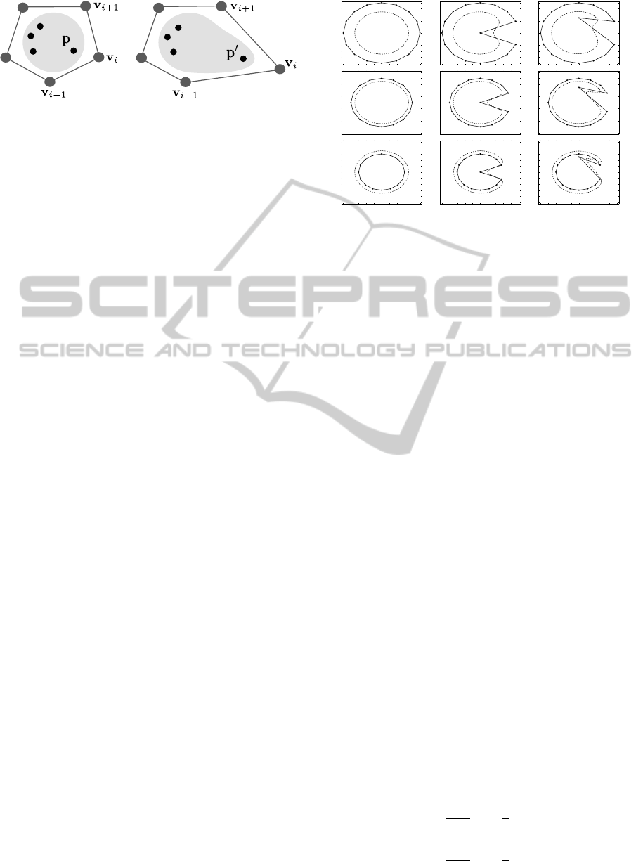
Figure 2: Example of the deformation of a region by means

of a closed polygon. From left to right: a polygon vertex v

is moved producing the consequent deformation of the re-

gion after applying the interpolation function. Pixels near

the moved vertex v

are affected more than pixels father

away due to the distance in the denominator of Equation (7).

point as described in this section. If a point v

of the

polygon is stretched in a particular direction, all the

points {p} follow the same direction with an associ-

ated weight given by ϕ

(p). The points p that are near

the moved vertex have higher weights (see denomina-

tor of Equation (7)) and thus suffer a larger “deforma-

tion” than the points which are farther away. Figure 2

and Figure 3 show an example to illustrate this phe-

nomena. In Figure 2 we schematically show how a

cloud of points can be deformed if one of the polygon

vertices is moved. Figure 3 depicts the inﬂuence of

the polygon vertex distance to a curve. In this exam-

ple mean value coordinates have been used to repre-

sent the curve with respect the closed polygon. On

the left column, the initial conﬁgurations are shown.

The polygon, made up of 16 vertices, is shown with a

solid line whereas the curve to deform with a dashed

line. From top to bottom, different initializations for

the polygon are shown: the ﬁrst two rows are asso-

ciated to polygon outside the curve whereas the last

row is associated to a polygon inside the curve. The

second and third column show how the curve is de-

formed when a control point of the polygon is moved.

As can be seen, the movement of the polygon pro-

duces a smooth deformation of the curve. The closer

the polygon to the curve, the higher the deformation

is applied to the curve.

In the three dimensional case a point p will be de-

scribed with respect to a closed surface made up of

triangles with vertices v

. The algorithm to compute

the mean value coordinates ϕ

(p) for a point p ∈ R

is described in (Ju et al., 2005). However, we would

like to point out here that Equations (6) and (9) are

still valid in the three dimensional case. Thus, it is

relatively easy to extend any two dimensional method

to the three dimensional case.

Equations (6) and (9) are the basis for the methods

we have developed in our work. The closed polygon

or surface can be interpreted as a cage that encloses

the object to deform. In the context of our work, the

control points are the cage vertices. The interior and

Figure 3: The curve deformation for different polygon

movements: external polygon (ﬁrst and second row) and

internal polygon (third row). The polygon is shown as solid

line and the evolving curve as dashed line.

exterior region points will be described with respect

to these cage points using the afﬁne coordinates. The

cage vertices will evolve according to the minimiza-

tion of an energy.

3 METHOD

Let us denote with I(p) : R

→ R a gray-level image,

where m = 2 (resp. m = 3) refers to a two-dimensional

(resp. three-dimensional) data. Let p be a point of R

and let us denote v = {v

,...,v

} the set of cage ver-

tices (or control points) associated to our parametriza-

tion. As commented previously, for m = 2 the cage

is a closed polygon whereas for m = 3 the cage is a

closed surface made up of triangles.

Let Ω

and Ω

be the set of pixels of the interior

and exterior, respectively, of the evolving interface C .

For each point p of Ω

and Ω

the afﬁne coordinates

are computed. When a cage vertex v

is moved, the

points inside Ω

and Ω

are deformed accordingly

(see Figure 2). Thus, in our work the evolving inter-

face does not need to be explicitly used to determine

Ω

and Ω

For simplicity we concentrate on the Chan and

Vese model. However, the method can be easily ex-

tended to other types of models. The Chan and Vese

model assumes that the gray-level values of pixels in-

side Ω

and Ω

can be modelled with different mean

values. The energy functional to minimize is:

E(v) =

|Ω

∑

p∈Ω

(I(p) − µ

)

|Ω

∑

p∈Ω

(I(p) − µ

)

. (10)

VISAPP2014-InternationalConferenceonComputerVisionTheoryandApplications

Figure 4: For a region-based energy term the contour

(dashed line) is evolved by minimizing an energy measured

in the interior region, Ω

, and the exterior region, Ω

. For

edge-based energies the contour is evolved by minimizing

an energy on the evolving interface.

where the mean gray-level value of Ω

with h ∈ {1,2}

is deﬁned as

|Ω

∑

p∈Ω

I(p), (11)

and | · | denotes the cardinal of the set. The energy

model is based on a direct discretization of the energy

functional of Equation (2). In order to minimize such

equation, one approach is to compute its gradient and

use it to drive the evolution of the interface to the min-

imum. This approach is called discretized optimiza-

tion approach in the context of energy minimization

problems (Kalmoun et al., 2011).

Let v

= (v

j,x

j,y

)

for m = 2 (resp. v

j,x

j,y

j,z

)

for m = 3) be the coordinates of a

cage vertex. The gradient of the energy with respect

to v

j,x

is given by

∂

∂v

j,x

(I(p) − µ

)

(I(p) − µ

)



∂I(p)

∂x

∂p

∂v

j,x

−

∂µ

∂v

j,x



. (12)

A similar expression is obtained for the partial deriva-

tive with respect to v

j,y

and v

j,z

. The partial deriva-

tives with respect to v

can be expressed in a compact

form as follows

∇

(I(p)−µ

)

= (I(p)−µ

)(ϕ

(p)∇I(p)−∇

(13)

where

∇

|Ω

∑

p∈Ω

(p)∇I(p). (14)

Thus, the gradient of E can be expressed as

∇

E(v) =

|Ω

∑

p∈Ω

(I(p) − µ

)(ϕ

(p)∇I(p) − ∇

)

|Ω

∑

p∈Ω

(I(p) − µ

)(ϕ

(p)∇I(p) − ∇

Note that for the computation of the gradient we have

assumed that the cardinal of sets Ω

and Ω

do not

depend on the cage vertex position. Indeed, as com-

mented before, Ω

and Ω

are made up of individual

pixels that deform as the vertex positions are moved.

As vertices move the corresponding evolving inter-

face may change its length (in two dimensional prob-

lems) or area (in three dimensional problems), but in

our implementation no pixels are added or removed

to Ω

and Ω

as the interface evolves. This approx-

imation may be correct if the deformation applied to

the cage is not grand. If the cage deforms with a big

zoom, it may be necessary to recompute, at a certain

iteration, the new set of pixels Ω

and Ω

. This idea

is similar to the one used in level sets implementation,

in which the distance function is used for the evolv-

ing function φ. Efﬁcient implementations re-initialize

φ to a distance function only every certain iterations.

4 IMPLEMENTATION

In this Section, we describe the implementation issues

associated to our proposed method.

Assume a gray-level image I and a mask Ω

are

available. The mask Ω

can be for instance a binary

image that is an approximation to the object we want

to segment. Thus, Ω

will be used as initialization

to our algorithm. In the case of medical images, for

instance, this mask can be obtained by means of a

registration of the image to be segmented with an at-

las. In some cases, the mask can be manually deﬁned

by the user. In this paper we will assume that Ω

a connected component. However, the method pre-

sented here is not restricted to this case. That is, Ω

may be composed of multiple connected components.

However, note that our method is not able to deal with

topological changes of Ω

Several choices are available to obtain the outer

pixels Ω

. For instance, Ω

can be taken as the set

Ω

= Ω \ Ω

, where Ω is the whole image support,

see Fig. 4. This is the way in which Ω

is deﬁned for

many level set approaches and is the case in our paper.

However, other approaches are possible. For instance,

only a band around Ω

may be taken. This is useful in

order to avoid taking pixels that are too far away from

ActiveContourSegmentationwithAffineCoordinate-basedParametrization

Ω

, see (Lankton and Tannenbaum, 2008). Note that

pixels of Ω

or Ω

may fall outside the polygon (2D)

or surface (3D) formed by the cage vertices.

Once the set of pixels of Ω

and Ω

have been

obtained, the afﬁne coordinates of the pixels p ∈ Ω

and p ∈ Ω

have to be computed. The afﬁne coordi-

nates are computed using the cage vertices v which

are assumed to be given as input. Recall that for each

point p ∈ R

, m = 2 or m = 3, a set of N coordinates

(i.e. ﬂoating point values) are obtained, where N is

the number of cage vertices. These coordinates only

have to be computed once, before the optimization al-

gorithm is initiated.

For a given E(v), the energy is minimized using

a gradient descent. The gradient method iteratively

updates v

k+1

from v

as follows

k+1

= v

+ αs

(15)

where s

is the so called search direction which is the

negative gradient direction s = −∇E(v

). The step α

is computed via a back-tracking algorithm. Starting

with an α = α

, the algorithm iteratively computes

E(v

+αs

) and reduces α until E(v

+αs

) < E(v

The computation of α

is a critical issue for good

performance of the algorithm. In this paper α

is au-

tomatically computed at each iteration k so that the

cage vertices move at most β pixels from its current

position. That is,

= max

{α|kv

k+1

− v

k ≤ β} j = 1 ...N (16)

where β is a user given parameter (usually set to 5 in

the experiments). The backtracking algorithm itera-

tively reduces the value of α until a value of α that

decreases the energy value is found. The gradient de-

scent stops when the backtracking reduces the α be-

low a threshold associated to a cage movement, for

instance 0.05 pixels.

For a given v, the corresponding “deformed” pixel

positions p of Ω

and Ω

are recovered using (9). The

energy E(v) and gradient ∇E(v) can be then com-

puted. Note that the recovered pixel positions p may

be non-integer positions. Hence, we apply linear in-

terpolation to estimate I(p) and ∇I(p) at such points.

In addition, those pixels that fall outside of the image

support are back projected to the image border (i.e.

pixels at the image border are assumed to extend to

inﬁnity).

To recover the ﬁnal position of the interface we

parametrize the interface at the beginning (before op-

timization starts) with respect to the cage vertices. Af-

ter convergence, the resulting interface can be easily

recovered by using Equation (9).

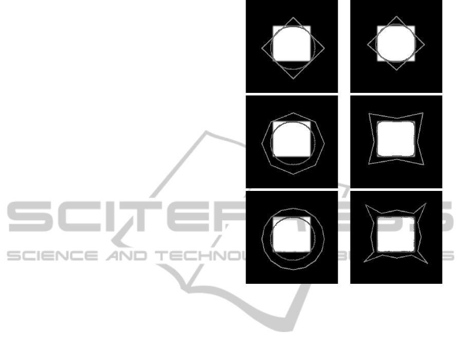
Figure 5: Results for a synthetic image using different num-

ber of cage points. Top, 4 cage points. Middle, 8 cage

points. Bottom, 16 cage points. On the left column the

initial images are shown, while the right correspond to the

results.

5 EXPERIMENTAL RESULTS

In this section we present the experimental results for

two and three dimensional segmentation problems. In

particular, we perform different experiments to show

different characteristics of the proposed segmentation

method: the inﬂuence of the number of cage vertex

selection, the importance of the cage shape, and the

performance on some real images.

5.1 Two Dimensional Segmentation

We begin with the two dimensional segmentation, that

is, the image I : R

→ R. We consider ﬁrst some syn-

thetic images, namely a square and a star, to analyze

the behaviour of our approach. For these experiments

Ω

is taken to be the whole interior of the evolving

interface and Ω

the whole exterior. We would like

to point out that in order to generate these images

the cage and the evolving contour has been painted

rounding the coordinates to nearest integers. Thus,

within the resulting images shown in this section there

may seem to be noisy boundaries.

VISAPP2014-InternationalConferenceonComputerVisionTheoryandApplications

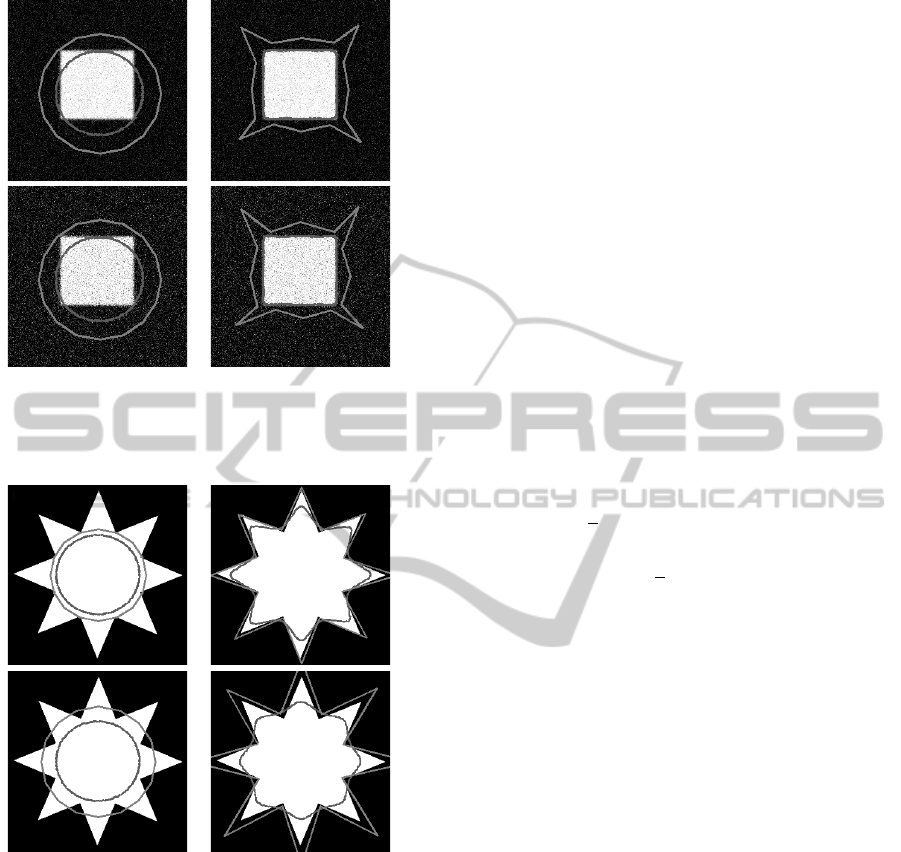
Figure 6: Results for a synthetic image and 16 cage points

using different levels of Gaussian noise. Top, noise variance

is σ

= 0.3. Bottom, σ

= 0.5, where the image gray-level

is assumed to be normalized to the range [0,1].

Figure 7: Results for a synthetic image with cages at dif-

ferent distances from the evolving contour. Images on the

left are the initial images and on the right are corresponding

results.

Figure 5 is devoted to show the inﬂuence of the

number of cage points to the segmentation result. The

initializations are shown on the left column and the

resulting segmentations are shown on the right. The

cages are drawn with light gray whereas the evolving

interface with dark gray. Experiments show how the

interface deforms when using 4, 8 and 16 cage points.

As can be seen, increasing the number of cage points

allows better adaptation to the shape of the object of

interest. The number of cage points inﬂuences the

regularization of the evolving contour.

Figure 6 shows the robustness of the method to

simple Gaussian noise. As expected, the model pro-

posed in Equation (10) is robust to Gaussian noise.

Figure 7 shows the effect of the cage distance to

the evolving interface. For both experiments the ini-

tial evolving interfaces are the same, but the cages are

created at a different distance from the evolving in-

terface: the distance on the top is smaller than the

bottom. The images on the left show initializations,

whereas the images on the right show the results. It

can be observed that the distance between the evolv-

ing interface and the cage plays an important role in

the deformations that can be applied to the evolving

interface. In addition, note that the result is inherently

regular (smooth ends instead of sharp ends) due to the

nature of the parametrization. Therefore no regular-

ization terms are needed in the energy function.

We now show results on real images. We have

compared our method with a level-set based Chan and

Vese implementation available in (Getreuer, 2012).

The code implements the following energy

E(C ) = µ Length(C ) +νArea(C )+

Ω

(I − µ

)

dx dy+

Ω

(I − µ

)

dx dy. (17)

The ﬁrst term of this energy controls the regularity of

the evolving contour C by penalizing the length. The

second term penalizes the enclosed area of C to con-

trol its side. The third and fourth terms are the terms

we use in our energy and penalize the discrepancy be-

tween the piecewise constant models µ

and µ

and

the input image.

The previous energy is implemented by means of

a level-set, please see details in (Getreuer, 2012). As

an example, we show in Figure 8 a segmentation re-

sult. The initialization of the level-set is performed

by using a checkerboard shape and is shown in the

middle Figure. The resulting segmentation is shown

in white on the right Figure and has been obtained

with the parameters µ = 0.25, ν = 0.0, λ

= 1.0 and

= 1.0. As can be seen, level-set based methods

are able to deal with topology changes and thus mul-

tiple connected components may be obtained in the

segmentation. Observe that here two contours have

been obtained as result: the contour around the ele-

phant and the one (small circle) over the head of the

elephant.

The results for the same image and two other real

images are shown in Figure 9. On the left, the initial-

ization is shown: the cage is drawn in black color and

the initial evolving contour in white. In the middle,

the resulting segmentation obtained with our method

is shown. On the right, the segmentation obtained

ActiveContourSegmentationwithAffineCoordinate-basedParametrization

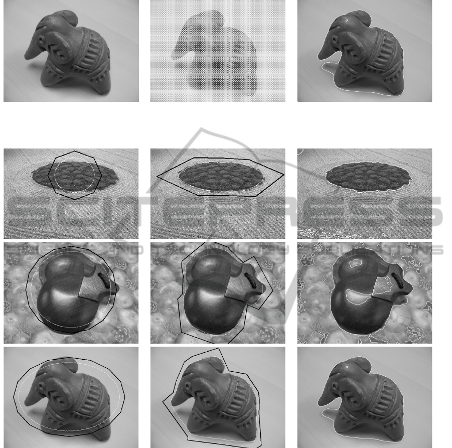
Figure 8: Example of level-set Chan and Vese segmentation. On the left, original image is shown. Initialization, a checker

board shape for the embedded function, is shown in the middle. On the right, resulting segmentation shows contour in white

color.

Figure 9: Results for some real images. On the left column, the initialization is shown: the cage is drawn in black color

whereas the evolving contour in white color. From top to bottom, the number of cage vertices used is 8, 16 and 16. In the

middle, the resulting segmentation obtained with our method is shown: the resulting cage and segmentation are again shown

in black and white, respectively. On the right, the resulting segmentation using a level-set based Chan and Vese segmentation

is shown.

with the Chan and Vese level-set method is shown.

The parameters that have been used for the latter are

µ = 0.25, ν = 0.0, λ

= 1.0, λ

= 1.0 for the second

and third row, whereas µ = 0.1, ν = 0.0, λ

= 1.0,

= 1.0 has been used for the ﬁrst row.

As can be seen, our method is able to obtain a

regular boundary without using any speciﬁc energy

term. Regularization is obtained thanks to the used

parametrization. In the level-set method, regulariza-

tion has to be explicitly introduced in the energy term.

On the other hand, the level-set method is able to deal

with topology changes (see the rather high number of

regions obtained in the images on the right column),

whereas our method does not. As commented before,

this limitation is a mild constraint in many applica-

tions, where the goal may be to simply segment one

connected object and thus the topological ﬂexibility

of the level sets is not needed.

VISAPP2014-InternationalConferenceonComputerVisionTheoryandApplications

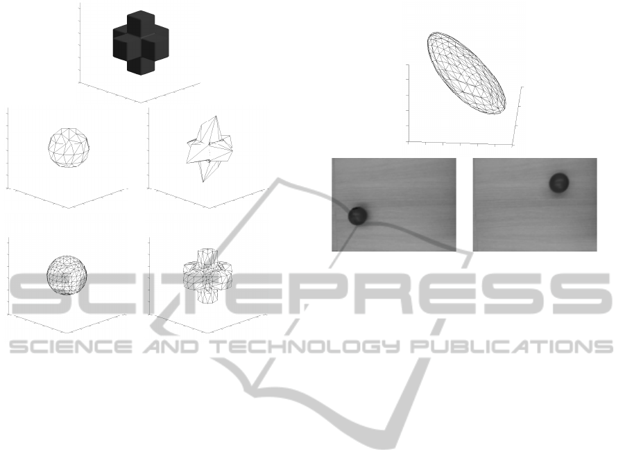
Figure 10: Results for a synthetic 3D image. Top, origi-

nal binary image. Middle left, the initial surface. The cage

has the same number of triangles but has a slightly higher

radius. Middle right, resulting surface after evolution. Bot-

tom, the same experiment is repeated but with a higher num-

ber of triangles for both the initial surface and the cage.

5.2 Three Dimensional Segmentation

We now show some examples for the three dimen-

sional segmentation problem. As commented before,

in this case the cage is a surface made up of triangles.

Figure 10 shows an example for a synthetic im-

age. The original image is shown on the top of the

Figure and represents a binary image with a cross.

The original surface is a ball which constructed using

the marching cube algorithm, is drawn on the middle

left. The cage is created from the previous surface just

by inﬂating it a bit (0.5 pixels). The surface is then

evolved using the proposed energy and the resulting

segmentation is drawn on the middle right. At the bot-

tom the same experiment is shown but in this case the

cage (as well as the mask) are modelled with a higher

number of vertices. As can be seen, the number of

vertices plays an important role in order to adapt the

evolving surface to the object of interest.

Finally, we show the result with real images, see

Figure 11. We have recorded a video in which a ball

moves along a line. The initial and end position of the

ball is shown on the bottom. The individual images

of the video are then stacked as a 3D image, and an

initial mask is created by deﬁning a 3D ball whose

center is approximately at the middle point joining the

Figure 11: Result for a real 3D image. Bottom, two of the

images of the video. Video images a stacked to form a 3D

image. Top, segmentation result for the moving ball.

initial and end position and whose radius (in 3D) is

the radius of the moving ball. On the top of Figure 11,

it can be seen the result after convergence has reached.

As can be observed, our method is able to properly

extract the “shape” of the 3D object formed by the

moving ball.

5.3 Computation Time

Currently, the code for 2D has been implemented in C

language whereas the 3D only has been implemented

in MATLAB. Regarding the 2D segmentation, the to-

tal amount of time spend by the algorithm is less than

one minute. This includes the computational time of

the mean value coordinates for all pixels of the im-

age and the gradient descent to evolve the contour.

With respect the 3D segmentation, the bottleneck is

currently at the computation of the mean value coor-

dinates for all the voxels of the volume, which may

take a long time. Gradient descent takes then about a

minute to converge.

Our method can be easily parallelized. Indeed,

two issues use most of the computation resources in

our approach, namely the interpolation of the image at

non-integer values (see Equation (9)) and the compu-

tation of the mean value coordinates. These two issue

will receive our focus of attention in future work.

6 CONCLUSIONS

In this paper, we have presented a parametrized ac-

tive contour approach for both two and three dimen-

sional segmentation problem. In our method the in-

ActiveContourSegmentationwithAffineCoordinate-basedParametrization

terface is evolved by moving a set of cage points.

In the two dimensional problem the cage is a closed

polygon whereas in the three dimensional problem

the cage is a closed surface (made up of triangles).

Mean value coordinates are used to parametrize the

points of the space, inside or outside the cage. Other

parametrization possibilities exist (such as harmonic

coordinates or Green coordinades), but we have se-

lected mean value coordinates since they are simple

to compute compared to other methods. Note that

the parametrization has an intuitive interpretation. By

moving a cage point, the associated points are moved

correspondingly. This allows to introduce into the

segmentation process the user interactivity: the user

may, for instance, manually move the control points

to the correct position so that the system automati-

cally learns from them.

In addition, within our framework, the regulariza-

tion of the evolving interface can be controlled via the

cage itself: the larger the distance of the cage to the

evolving contour, the higher the contour regulariza-

tion. Thus, there is really no need to include regular-

ization terms within the energy.

Our framework is suitable for the implementa-

tion of discrete energies, both region-based and edge-

based terms, although we have shown here only the

application to a region-based energy, namely the clas-

sical Chan and Vese one.

Morover, we think that our method can be easily

embedded in a shape-constrained approach, that is, an

approach in which the movement of the cage is con-

strained so as to ensure certain shapes for the evolving

contour. Our future work is to apply our method for

3D medical image segmentation problems and paral-

lelize the method to improve its speed.

ACKNOWLEDGEMENTS

Q. Xue would like to acknowledge support from Eras-

mus Mundus BioHealth Computing, L. Igual and L.

Garrido by MICINN projects, reference TIN2012-

38187-C03-01 and MTM2012-30772 respectively.

REFERENCES

Barbosa, D., Dietenbeck, T., Schaerer, J., D’hooge, J., Fri-

boulet, D., and Bernard, O. (2012). B-spline explicit

active surfaces: an efﬁcient framework for real-time

3D region-based segmentation. IEEE Transactions on

Image Processing, 21(1):241–251.

Caselles, V., Kimmel, R., and Sapiro, G. (1997). Geodesic

active contours. International Journal of Computer

Vision, 22:61–79.

Chan, T. and Vese, L. (2001). Active contours without

edges. IEEE Trans. on Imag. Proc., 10(2):266–277.

Coquillart, S. (1990). Extended free-form deformation:

a sculpturing tool for 3d geometric modeling. SIG-

GRAPH, 24(4):187–196.

Faloutsos, P., van de Panne, M., and Terzopoulos, D.

(1997). Dynamic free-form deformations for anima-

tion synthesis. IEEE Transactions on Visualization

and Computer Graphics, 3(3):201–214.

Floater, M. S. (2003). Mean value coordinates. Computer

Aided Geometric Design, 20(1):19–27.

Getreuer, P. (2012). Chan-vese segmentation. Image Pro-

cessing On Line.

Gouraud, H. (1971). Continuous shading of curved sur-

faces. IEEE Transactions on Computers, C-20(6):623

– 629.

Hormann, K. and Floater, M. (2006). Mean value coordi-

nates for arbitrary planar polygons. ACM Transac-

tions on Graphics, 25(4):1424–1441.

Hormann, K. and Greiner, G. (2000). Continuous shading

of curved surfaces. Curves and Surfaces Proceedings

(Saint Malo, France), pages 152 – 163.

Jacob, M., Blu, T., and Unser, M. (2004). Efﬁcient energies

and algorithms for parametric snakes. IEEE Transac-

tions on Image Processing, 13(9):1231–1244.

Joschi, P., Meyer, M., DeRose, T., Green, B., and Sanocki,

T. (2007). Harmonic coordinates for character articu-

lation. In SIGGRAPH.

Ju, T., Schaefer, S., and Warren, J. (2005). Mean value coor-

dinates for closed triangular meshes. In Proceedings

of ACM SIGGRAPH, volume 24, pages 561–566.

Kalmoun, M., Garrido, K., and Caselles, V. (2011). Line

search multilevel optimization as computational meth-

ods for dense optical ﬂow. SIAM Journal of Imaging

Sciences, 4(2):695–722.

Kass, M., Witkin, A., and Terzopoulos, D. (1988). Snakes:

Active contour models. International Journal of Com-

puter Vision.

Lankton, S. and Tannenbaum, A. (2008). Localizing region-

based active contours. IEEE Transactions on Image

Processing, 17(11):2029–2039.

Lipman, Y., Kopf, J., Cohen-Or, D., and Levin, D. (2007).

GPU-assisted positive mean value coordinates for

mesh deformations. In Eurographics Symposium on

Geometry Processing.

Lipman, Y., Levin, D., and Cohen-Or, D. (2008). Green

coordinates. In SIGGRAPH.

Michailovich, O., Rathi, Y., and Tannenbaum, A. (2007).

Image segmentation using active contours driven by

the Bhattacharyya gradient ﬂow. IEEE Transactions

on Image Processing, 16(11):2787–2801.

Rousson, M. and Deriche, R. (2002). A variational frame-

work for active and adaptative segmentation of vec-

tor valued images. In Proceedings of the Workshop

on Motion and Video Computing, pages 56–61. IEEE

Computer Society.

Rueckert, D., Sonoda, L., Hayes, C., Hill, D., Leach,

M., and Hawkes, D. (1999). Nonrigid registration

using free-form deformations: application to breast

MR images. IEEE Transactions on Medical Imaging,

18(8):712–721.

VISAPP2014-InternationalConferenceonComputerVisionTheoryandApplications