Regional SVM Classifiers with a Spatial Model for Object Detection

Zhu Teng

, Baopeng Zhang

, Onecue Kim

and Dong-Joong Kang

School of Computer and Information Technology, Beijing Jiaotong University, No.3 Shang Yuan Cun,

Hai dian District Beijing, China

Department of Mechanical Engineering, Pusan National University, Busandaehak-ro 63beon-gil Geumjeong-gu,

Busan, South Korea

Keywords: Regional SVM, Object Detection, Spatial Model.

Abstract: This paper presents regional Support Vector Machine (SVM) classifiers with a spatial model for object

detection. The conventional SVM maps all the features of training examples into a feature space, treats

these features individually, and ignores the spatial relationship of the features. The regional SVMs with a

spatial model we propose in this paper take into account a 3-dimentional relationship of features. One-

dimensional relationship is incorporated into the regional SVMs. The other two-dimensional relationship is

the pairwise relationship of regional SVM classifiers acting on features, and is modelled by a simple

conditional random field (CRF). The object detection system based on the regional SVM classifiers with the

spatial model is demonstrated on several public datasets, and the performance is compared with that of other

object detection algorithms.

1 INTRODUCTION

Detecting an object of a category is very challenging

in the computer vision area due to the significant

changes in object color, illumination, viewpoint,

large intra-class variability in shape, appearance,

pose, and complex background clutter and

occlusions. As it is one of the most significant tasks

in this field, it has been studied by many researchers

for decades, and many successful results have been

reported. A detector that localizes objects in an

image was realized by some learning algorithms in

many studies. The learning method used in object

detection can be a boosting algorithm (Alexe et al.,

2010), a Support Vector Machine (SVM) (Scholkopf

and Smola, 2002), a transformation of any of them

(Opelt et al., 2006) or a combination of some of

them (Song et al., 2011). In this paper, we propose

the multiple regional SVM classifiers to enhance the

performance of the SVM classifier and focus on

modelling the spatial relationship of these regional

SVM classifiers.

The spatial relationship has been taken into

consideration in many works. In (Tagare et al.,

1995), the spatial relation of similar patches was

described, and a model of the spatial relation

between parts was learnt in (Kumar and Hebert,

2006, David J. Crandall, 2006, David Crandall,

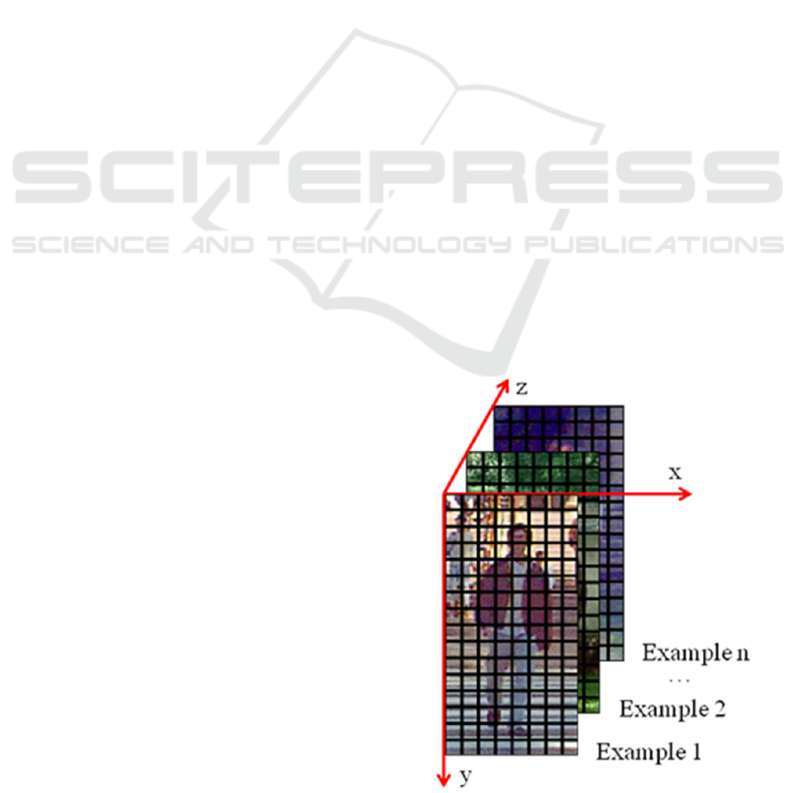
Figure 1: Spatial relationship. View the cell features of

training examples in a 3D space. The spatial relationship

along z axis is encoded by the regional SVM classifiers,

and the spatial relationship along axis x and axis y is

delineated by the spatial model.

372

Teng Z., Zhang B., Kim O. and Kang D..

Regional SVM Classiﬁers with a Spatial Model for Object Detection.

DOI: 10.5220/0004679003720379

In Proceedings of the 9th International Conference on Computer Vision Theory and Applications (VISAPP-2014), pages 372-379

ISBN: 978-989-758-004-8

 2014 SCITEPRESS (Science and Technology Publications, Lda.)

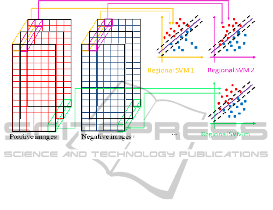
Figure 2: The training of regional SVMs. There are m feautres in an image, so m regional SVMs should be learnt. In each

feature space of regional SVMs, a red point denotes for a positive feature, a blue square indicates a negative feature, and

there are 2n features for each feature space.

2005). Others encoded the spatial relationship in a

graphical model such as the Bayesian model

(Bogdan et al., 2010), a pictorial structure (Fischler

and Elschlager, 1973), a tree model (Long (Leo) Zhu,

2010), etc. Most of these approaches require the

association of a label to a part in order to learn the

model, and it becomes unsound if some of the parts

are missing or undetected. In addition, sometimes

good part structures should be carefully selected

(Felzenszwalb et al., 2010). In contrast, we explore

the spatial relationship of regional SVM classifiers

acting on cell features, which is a lower level

description compared with the part description, and

it requires no labels of parts.

We describe the spatial relationship in Fig. 1.

Assume the cell features (split training examples

into cells) for training are viewed in a 3D space, the

spatial relationship along the axis z is incorporated

into the regional SVM classifiers, and the spatial

relationship along the axis x and axis y (or on the x-

y plane) is described as a pairwise relationship of

regional SVM classifiers modelled by a simple

conditional random field (CRF).

The contributions of this paper include: 1)

construction of regional SVM classifiers to boost the

performance of SVM classifier; 2) modelling of the

pairwise relationship of regional SVM classifiers by

CRF. The conventional SVM training maps all the

features of positive and negative training images into

a feature space and finds a decision plane. In

contrast, we build several regional SVMs, and the

training data for each SVM are the features from

different instances at the same location. The number

of regional SVMs is determined by the number of

cells in one instance. The training time of multiple

regional SVMs is largely decreased compared with

that of the conventional SVM, and above all,

regional SVM classifiers improve the performance

because each regional SVM classifier encloses a

spatial relationship among examples.

The rest of the paper is arranged as follows. The

regional SVMs are described in Section 2, and the

spatial model based on CRF that expresses the

pairwise relationship of regional SVM classifiers is

illustrated in Section 3. Experiments and discussions

are presented in Section 4, and conclusions follow in

Section 5.

2 REGIONAL SVM CLASSIFIERS

We will first give the main idea of the regional

SVMs in Section 2.1. The prediction using the

learned regional SVM classifiers is illustrated in

Section 2.2.

…

RegionalSVMClassifierswithaSpatialModelforObjectDetection

373

2.1 Definition of Regional SVMs

The regional SVMs are constructed by multiple local

SVMs, each encoding the patterns of features from

different spatial districts. The features from different

images with the same relative location are collected

for each individual SVM of regional SVMs. The

feature utilized here is cell-based features (such as

HOG (Dalal and Triggs, 2005, Felzenszwalb et al.,

2008) or LBP (Ojala et al., 1996), that is, several

features can be extracted from a single image. The

number of SVMs in the regional SVMs is the

number of cell features in one single image. The

implementation for an individual SVM of regional

SVMs is the same as that for the conventional SVM.

Assume we have n positive images and n

negative images, denoted by {PI

,PI

,…,PI

} and

{NI

,NI

,…,NI

}, respectively. We also presume

there are m features extracted from one image.

Features for the i

positive image and the i

negative

image are described by

},...,,{

iii

PIPI

XXX

and

},...,,{

iii

NINI

XXX

, respectively.

The conventional SVM maps all the features of

positive and negative images into a feature space,

and then the conventional SVM model is trained

using the feature set

]},1[],,1[|,{ mjniXX



. The regional

SVMs we propose train m SVMs (as shown in Fig.

2). Each SVM of regional SVMs delineates the

characteristics of the object with different spatial

locations. The training set for the i

SVM

(

mi ,...,1

) is defined as

},...,,,,...,,{

2121 nn

XXXXXX

The union of the training data of all the regional

SVMs is the same with the training data of the

conventional SVM, but the patterns for each SVM of

the regional SVMs are reconstituted. To train each

individual SVM of the regional SVMs, the LibSVM

(Chang and Lin, 2011) is employed in our program.

2.2 Prediction of Regional SVM

Classifiers

The prediction of the regional SVMs for a detection

window is reached by all the SVM models

constructed in the training of regional SVMs. The

relative location of each feature in the detection

window can be perceived, and as we denote the

features in the detection window by

},...,,{

xxx

, the subscripts 1,2,…,m

indicate the relative location of features in the

current window. The decision on the detection

window is made with Eq. (1), which suggests that

the detection window contains an object if the

confidence is positive; otherwise, the detection

window is determined to be a non-object window.











)b)x,K(xαysgn(

)b)φ(xsgn(wconfidence

(1)

where



, and

b are parameters of the f

SVM model in the regional SVMs. s indicates the

number of support vectors and K is the kernel

function, we use the linear kernel in the program.

We can see from Eq. (1) that the prediction of a

detection window in the regional SVMs is associated

with both the relative location of the feature to be

tested in the detection window and the regional

SVM classifier, as each cell feature of the detection

window is estimated by the corresponding regional

SVM classifier. In other words, if the same feature

has different locations in different windows, the

prediction result of the feature in different windows

could also be different.

3 A SPATIAL MODEL BASED ON

CRF

In this section, we introduce the spatial model that

encodes the pairwise relationship (spatial

relationship along axes x and y in Fig. 1) of regional

SVM classifiers acting on features. The spatial

model is built based on the CRF (Koller and

Friedman, 2009) and predicts a binary label Y that

suggests the category of a detection window, given

an observed feature vector X. The pairwise

relationship is incorporated in the feature vector X.

The model we employ in our formulation is a

simple CRF. The conditional probability P(Y|X) is

formulated by Eq. (2) and θ is the parameter we

want to estimate.

)1(

)

()

()|(















(2)

The parameter estimation approach we use to

learn the model of the conditional probability

P(Y|X) is the maximum likelihood estimation.

VISAPP2014-InternationalConferenceonComputerVisionTheoryandApplications

374

Figure 3: Pairwise relationship of regional SVM classifiers

acting on cell features.

Assume that the training dataset is denoted by

}1),,{(

CcyD



x , given

C training

examples, in the learning process, we need to

estimate θ* that minimizes the negative log

likelihood of the training data L

-regularization

expressed in Eq. (3).

* arg min log( ( : ))

arg min log( ( | ; ))













 





x θ

θθ

(3)

Our learning problem is transformed to an

optimization problem, and to perform this

optimization, the stochastic gradient descent

algorithm (Koller and Friedman, 2009) is utilized.

The update rule is presented in Eq. (4).

:[log((|;)]

[ (1 ) log( ) log(1 ) ]

()]

ye e















  

     

  



θθ

θθ θ θ

θθ

(4)

To this point, we explained the parameter estimation

process of our spatial model, and the only thing we

have not yet reported is how to express the feature

. The feature x

in our spatial model is required to

enclose the pairwise relationship of regional CRF

classifiers acting on cell features in one detection

window or one training example (we will call it the

specified window hereafter). It is defined as a row of

confidences that the regional SVM classifiers predict

on each cell feature in the specified window, so the

feature x

represents the specified window. Since the

number of the regional SVM classifiers (denoted by

m) is equal to the number of cell features defined in

a specified window, the feature x

for the specified

window has a size of 1*m

to describe the pairwise

relationship between regional SVM classifiers acting

on cell features (as shown in Fig. 3). We use SVM

(

w ,

b ) to denote the i

SVM of the regional SVM

classifiers, and represent the feature of the j

cell of

the specified window as

, and assume there are

m cells in one specified window. A feature matrix

cij

, which has the size of m*m, can be calculated by

Eq. (5). The feature x

of our spatial model is gained

by reshaping matrix X

cij

to a row vector.

),(

cellSVMconfidence



cij

(5)

After learning all the parameters of the spatial

model, a prediction approach is required in order to

make a decision on a new feature x

cnew

. We judge

the new feature as positive if the possibility of Y=1

is larger than the possibility of Y=0; otherwise, the

new feature is settled as negative. The verdict rule is

articulated by Eq. (6) and the derivation of this

verdict rule is explained in Eq. (7).

(1 )

cnew

ysigne







cnew

(6)

(1|)(0|)

cnew cnew

Py Py







 

cnew cnew

(7)

4 EXPERIMENTS

Two kinds of experiments are reported in this

section. The comparison between the regional SVMs

and the SVM is demonstrated with experiments in

Section 4.1. The experiments for the spatial model

and detecting objects in images are revealed in

Section 4.2. All of the experiments are executed on

an Intel(R) i5 2.80GHz desktop computer.

4.1 Performance Comparison between

Regional SVMs and the

Conventional SVM

The performance of regional SVMs and the SVM

(Hsu et al., 2003) is estimated and compared on two

public datasets, MIT pedestrian dataset and UIUC

Image Database for Car Detection. Two kinds of

widely used features are involved, and the training is

executed in a 5-fold cross validation, so the final

accuracy is the average accuracy of the five runs.

Experimental setting. The HOG feature is

employed in the experiment on the MIT pedestrian

dataset. The cell size of the HOG feature is 8*8

pixels. We operate the LBP feature in the

experiment of the UIUC Image Database for Car

Detection, and the cell size of the LBP feature is

defined as 16*16 pixels. The CRF based spatial

model is not used in this experiment for a fair

comparison.

RegionalSVMClassifierswithaSpatialModelforObjectDetection

375

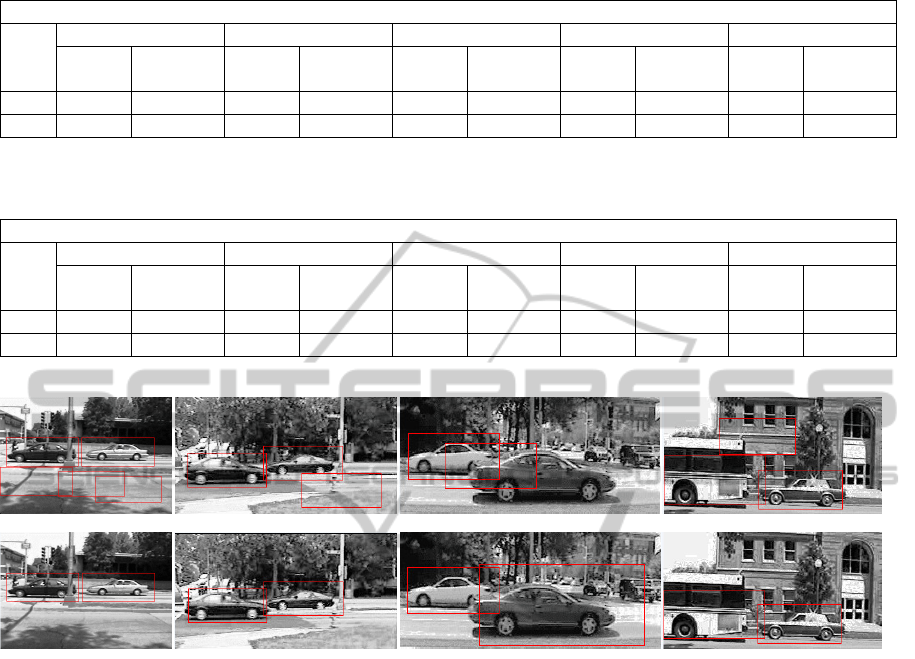
Table 1: Comparison results between regional SVMs and the SVM on the MIT Pedestrian Dataset for human detection.

MIT pedestrian dataset 5-fold cross validation HOG feature

1000 examples 800 examples 600 examples 400 examples 200 examples

SVM Regional

SVMs

SVM Regional

SVMs

SVM Regional

SVMs

SVM Regional

SVMs

SVM Regional

SVMs

acc 0.6241 0.7528 0.6256 0.7487 0.6210 0.7431 0.6185 0.7307 0.6342 0.7170

time 4931 s 29.41s 3151s 22.49s 1721s 15.51s 748.2s 7.672s 110.7s 3.566s

Note: The bold number indicates the best performance.

Table 2: Comparison results between regional SVMs and the SVM on the UIUC Image Database for car detection.

UIUC Image Database for Car Detection 5-fold cross validation LBP feature

1000 examples 800 examples 600 examples 400 examples 200 examples

SVM Regional

SVMs

SVM Regional

SVMs

SVM Regional

SVMs

SVM Regional

SVMs

SVM Regional

SVMs

acc 0.6837 0.7464 0.6848 0.7389 0.6886 0.7368 0.6998 0.7435 0.7154 0.7350

time 286.6s 20.44s 180.5s 14.01s 101.5s 7.394s 43.38s 3.640s 9.723s 1.258s

Note: The bold number indicates the best performance.

Figure 4: Comparisons of several shots that are processed by our object detection system with and without the spatial model

on the UIUC Car Dataset. Top row: Results of our object detection system without the spatial model. Bottom row: Results

of our object detection system with the spatial model.

Table 1 epitomizes the accuracy and time cost of

two methods testing on the MIT Pedestrian Dataset.

We see that the accuracy of the regional SVM

classifiers is improved by at least 10%, compared

with the results processed by the SVM. The

performance is enhanced a little in the experiment of

200 examples, but not as much as the other

experiments with more examples, because of the

limited number of training samples. Generally, for

the regional SVMs, the more training examples used

in the experiment, the better the accuracy

performance. The computational time we reveal in

the table contains the training time and predicting

time for five runs of cross validations. It is clear

from Table 1 that the training of regional SVMs is

dozens of times faster than that of the SVM despite

of the number of training examples that are used.

Table 2 discloses the results on the UIUC Image

Database. With the results of Table 2, a similar

conclusion can be reached. To summarize, the

regional SVMs is superior to the SVM algorithm on

both the accuracy performance and time

performance.

4.2 Object Detection in Images

The object detection experiments are first executed

on the UIUC Image Database for Car Detection,

which contains training images, single-scale test

images, and multi-scale test images. Since multi-

scale test images are more difficult than the single-

scale test images, we use the single-scale test images

as the validation dataset and examine our algorithm

on the multi-scale test images. The feature we use to

represent images is a 31-dimensional HOG feature,

and we employ a pyramid framework to detect

multiple scales of objects. The confidences gauged

by regional SVMs and the spatial model are fused by

the weighted average, and the weights are reckoned

on the validation dataset. The training process is

VISAPP2014-InternationalConferenceonComputerVisionTheoryandApplications

376

performed twice to explore hard negative examples.

In the first iteration, cropped training images with a

fixed size are used to train initial regional SVMs,

and then hard negative examples are explored by

detecting the original training negative files rather

than cropped training negative examples

(Felzenszwalb et al., 2010). The hard negative

examples are added to the negative training set to

conduct the second round of training. The process of

detecting objects using our proposed algorithm

consists of four steps (given a test image): 1)

pyramid feature extraction; 2) predictions by

regional SVMs; 3) confidences estimated by the

spatial model; 4) non-maximum suppression. The

non-maximum suppression is employed to deal with

the situation in which multiple overlapping

detections for each instance of an object are

obtained. The bounding box with the highest

confidence is reported among bounding boxes

overlapping at least 50%.

Fig. 4 presents comparisons of several shots that

are processed by our object detection system with

and without the spatial model. It is clear that the

spatial model greatly improves the performance. The

performance on the entire dataset is assessed by the

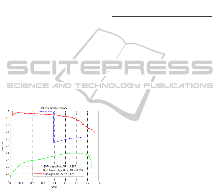
Figure 5: Precision-recall curve on the Caltech Airplanes

Dataset.

precision, recall and F-measure of the testing results,

and Table 3 presents the results of ours compared

with the Neighborhood Suppression Algorithm

(NSA) and the Repeated Part Elimination Algorithm

(RPEA) of (Agarwal et al., 2004), which have also

evaluated the performance on the multi-scale test

images of the UIUC Database. The results of Table

3 demonstrate that our algorithm achieves a

performance (F-measure) that is almost 20% better

than the performance of the NSA and RPEA. Note

that the best F-measure of these two algorithms

reported in (Agarwal et al., 2004) is referred to in

Table 3.

Table 3: Performance on the multi-scale test images of the

UIUC Image Database for Car Detection.

SA RPEA Ours

Recall 38.85% 39.57% 66.91%

Precision 49.09% 49.55% 60.00%

F-measure 43.37% 44.00% 63.27%

We also evaluate our proposed algorithm on the

Caltech Airplanes dataset consisting 1074 images,

which are divided into a training set (500 images),

an validation set (74 images) and a test set (500

images). The training process is similar to that

applied on the Car Dataset and the performance is

evaluated by the precision-recall curve (Everingham

and Zisserman, 2007) as shown in Fig. 5 (some of

the detection results are shown in Fig. 6). The

comparison methods include the SVM method that

employs the HOG feature and part-based algorithm

(Felzenszwalb et al., 2010), and our algorithm gives

the best average precision (AP) (Everingham and

Zisserman, 2007) and a relatively better performance.

5 CONCLUSIONS

This paper presents the regional SVM classifiers

with a spatial model to describe the 3D (axes x, y, z

in Fig. 1) spatial relationship of features, which is

ignored by the conventional SVM. Regional SVM

classifiers encode the spatial relationship along axis

z, and the spatial model incorporates the spatial

relationship along axes x and y. We demonstrate

regional SVM classifiers with the spatial model

using diversified features in various categories, and

the experiments establish that the regional SVM

classifiers do enhance the performance of the SVM

classifier and the spatial model improves the

performance of the object detection system. The

experiments on the benchmark datasets show that

our system has a relatively better performance

compared with other object detection algorithms.

ACKNOWLEDGEMENTS

This work was financially supported by the Basic

Science Research Program through the National

Research Foundation of Korea (NRF) funded by the

Ministry of Education, Science and Technology

RegionalSVMClassifierswithaSpatialModelforObjectDetection

377

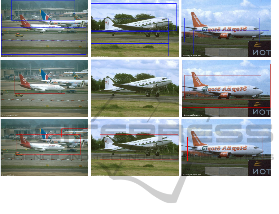
Figure 6: Results on the Caltech Airplanes dataset. Top row: processed by the conventional SVM; Middle row: processed

by the part-based algorithm (Felzenszwalb et al., 2010); Bottom row: processed by our algorithm.

(2011-0027213 and 2011-0017228), and also

partially supported by Natural Science Foundation

of China (61300175 and 61301185) and

Fundamental Research Funds for the Central

Universities of the Ministry of Education of China

with grant number 2012JBM033.

REFERENCES

Moore, R., Lopes, J., 1999. Paper templates. In

TEMPLATE’06, 1st International Conference on

Template Production. SCITEPRESS.

Smith, J., 1998. The book, The publishing company.

London, 2

edition.

Bernhard Scholkopf, Alexander J. Smola, 2002. Learning

with kernels: Support Vector Machines,

Regularization, Optimization, and Beyond, The MIT

Press.

Andreas Opelt, Axel Pinz, Andrew Zisserman, 2006.

Incremental learning of object detectors using a visual

shape alphabe, In Proc. IEEE Conf. Computer Vision

and Pattern Recognition, vol. 1, pp. 3-10.

Zheng Song, Qiang Chen, Zhongyang Huang, Yang Hua,

Shuicheng Yan, 2011. Contextualizing Object

Detection and Classification, In IEEE Conf. on

Computer Vision and Pattern Recognition (CVPR).

Tagare H., Vos F., Jaffe C.C., Duncan J.S., 1995.

Arrangement: A spatial relation between parts for

evaluating similarity of tomographic section, In IEEE

Trans. PAMI, 17 (9), 880-893.

Bogdan Alexe, Thomas Deselaers, Vittorio Ferrari, 2010.

What is an object? In Proc. CVPR.

Martin A. Fischler, Robert A. Elschlager, 1973. The

representation and matching of pictorial structures, In

IEEE Transactions on Computers, Vol. c-22, No. 1.

Long (Leo) Zhu, Yuanhao Chen, Alan Yuille, William

Freeman, 2010. Latent Hierarchical Structural

Learning for Object Detection, In Proc. IEEE

Computer Vision and Pattern Recognition (CVPR).

Sanjiv Kumar, Martial Hebert, 2006. Discriminative

random fields: A discriminative framework for

contextual interaction in classification, In Int. J.

Comput. Vis., vol. 68, no. 2, pp.179 -201.

David J. Crandall and Daniel P. Huttenlocher, 2006.

Weakly Supervised Learning of Part-Based Spatial

Models for Visual Object Recognition, In Proc.

ECCV, pages I: 16-29.

David Crandall, Pedro Felzenszwalb, Daniel Huttenlocher,

2005. Spatial Priors for Part-Based Recognition using

Statistical Models, In Proc. IEEE Conf. Computer

Vision and Pattern Recognition.

Navneet Dalal and Bill Triggs, 2005. Histograms of

Oriented Gradients for Human Detection, In Proc.

IEEE Conf. Computer Vision and Pattern Recognition.

VISAPP2014-InternationalConferenceonComputerVisionTheoryandApplications

378

T. Ojala, M. Pietikäinen, and D. Harwood, 1996. A

Comparative Study of Texture Measures with

Classification Based on Feature Distributions, In

Pattern Recognition, vol. 29, pp. 51-59.

Daphne Koller, Nir Friedman, 2009. Probabilistic

Graphical Models: Principles and Techniques -

Adaptive Computation and Machine Learning, The

MIT Press.

Pedro F. Felzenszwalb, Ross B. Girshick, David

McAllester, and Deva Ramanan, 2010. Object

Detection with Discriminatively Trained Part-Based

Models, In IEEE Trans. PAMI, Vol. 32, No. 9.

P. Felzenszwalb, D. McAllester, and D. Ramanan, 2008.

A Discriminatively Trained, Multiscale, Deformable

Part Model, In Proc. IEEE Conf. Computer Vision and

Pattern Recognition.

C.-C. Chang and C.-J. Lin, 2011. LIBSVM : a library for

support vector machines, In ACM Transactions on

Intelligent Systems and Technology, 2:27:1--27:27.

Software available at http://www.csie.ntu.edu.tw/

~cjlin/libsvm.

Chih-Wei Hsu, Chih-Chung Chang, and Chih-Jen Lin,

2003. A Practical Guide to Support Vector

Classification, Technical Report, Taipei.

M. Everingham, A. Zisserman, C.K.I., Williams and L.

Van Gool, 2007. The PASCAL Visual Object Classes

Challenge 2007 (VOC 2007) Results. Available at:

http://pascallin.ecs.soton.ac.uk/challenges/VOC/voc20

07/.

Shivani Agarwal, Aatif Awan, and Dan Roth, 2004.

Learning to detect objects in images via a sparse, part-

based representation, In IEEE Transactions on Pattern

Analysis and Machine Intelligence, 26(11):1475-1490.

RegionalSVMClassifierswithaSpatialModelforObjectDetection

379