Oriented Half Gaussian Kernels and Anisotropic Diffusion

Baptiste Magnier and Philippe Montesinos

Ecole des Mines d’ALES, LGI2P, Parc Scientiﬁque G. Besse, 30035 N

ımes Cedex, France

Keywords:

Half Anisotropic Gaussian Kernel, Diffusion PDEs.

Abstract:

Nonlinear PDEs (partial differential equations) offer a convenient formal framework for image regularization

and are at the origin of several efﬁcient algorithms. In this paper, we present a new approach which is based

(i) on a set of half Gaussian kernel ﬁlters, and (ii) a nonlinear anisotropic PDE diffusion. On one hand, half

Gaussian kernels provide oriented ﬁlters whose ﬂexibility enables to detect edges with great accuracy. On the

other hand, a nonlinear anisotropic diffusion scheme offers a means to smooth images while preserving ﬁne

structures or details, e.g. lines, corners and junctions. Based on the calculus of the gradient magnitude and

two diffusion directions, we construct a diffusion control function able to achieve precise image regulariza-

tion. Some quantiﬁed experimental results compared to existing PDEs approaches and a discussion about the

parameterizing of the method are presented.

1 A FRAMEWORK OF

ANISOTROPIC DIFFUSION

WITH PDE

Obtain regularized versions of noisy, corrupted or de-

graded images caused for example by compression ar-

tifacts is a difﬁcult task in image processing. How-

ever, preserving signiﬁcant internal structures is a

ﬁeld that has largely beneﬁted from techniques of Par-

tial Differential Equations (PDE) (Aubert and Korn-

probst, 2006; Magnier and Montesinos, 2013). PDEs

belong to one of the most important part of mathe-

matical analysis and are closely related to the physi-

cal world. In this context, images are considered as

evolving functions of time and a regularized image

can be seen as a version of the original image at a

special stage. Thereby, PDEs methods smooth locally

the image following one or several directions which

are different in each point of the image. In this paper,

let us note I : Ω → R, (Ω ⊂ R

) a grey level image

with I(x,y) corresponding to the pixel intensity of co-

ordinates (x, y). Considering I

the original image,

the general evolution model can be formally written

in the following form:



∂I

∂t

(x,y,t) = F (I(x,y,t))

I(x, y,0) = I

(x,y)

(1)

where F is a given image processing algorithm, pre-

serving edges having high gradient. F represents a

function of the original image I

and its ﬁrst and

second order spatial derivatives (Caselles and Morel,

1998).

It should be noted that Koenderink (Koenderink,

1984) was the ﬁrst to underline the equivalence be-

tween the convolution with a Gaussian kernel of stan-

dard deviation

√

2t and the solution of the PDE de-

scribing the heat diffusion, at a time t. This smooth-

ing process, called isotropic diffusion, is known to

smooth noise but blur edges, leading to loose image

structures. In order to regularize images by control-

ling the diffusion, Perona and Malik (Perona and Ma-

lik, 1990) have proposed a model described by the

following equation:

∂I

∂t

(x,y,t) = div(g(k∇Ik) ·k∇Ik) (2)

where div represents the divergence operator and

g(s) : [0,+∞[→]0,+∞[ a decreasing function satisfy-

ing g(0) = 1 and g(+∞) = 0, this function could be

chosen as g (k∇Ik) = e



−

k∇Ik



, with K ∈ R a con-

stant that can be assimilated to a gradient threshold or

a diffusion barrier.

The decomposition of the eq. 2 with the second

derivatives of I in orthogonal directions (ξ ⊥ η) re-

spectively in the edge direction called ξ and in the

gradient direction labelled η =

∇I

k∇Ik

enables to under-

stand the diffusion behavior (Kornprobst et al., 1997):

∂I

∂t

(x,y,t) = c

·I

ξξ

+ c

·I

ηη

(3)

Magnier B. and Montesinos P..

Oriented Half Gaussian Kernels and Anisotropic Diffusion.

DOI: 10.5220/0004679500730081

In Proceedings of the 9th International Conference on Computer Vision Theory and Applications (VISAPP-2014), pages 73-81

ISBN: 978-989-758-003-1

 2014 SCITEPRESS (Science and Technology Publications, Lda.)

where (I

ξξ

ηη

) =



∂

∂ξ

∂

∂η



, c

and c

are coefﬁ-

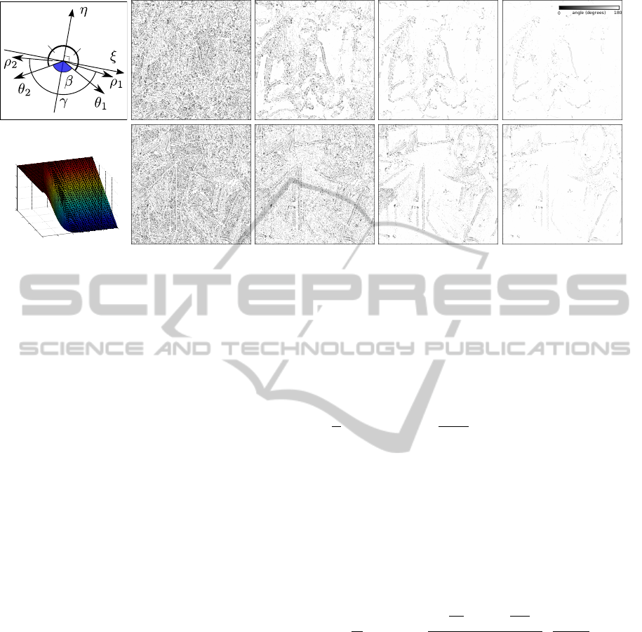
cients tuning the diffusion (diagrammed in Fig. 1(a)).

When c

ξξ

= c

ηη

= 1, the eq. 3 is equivalent to the

heat equation (Koenderink, 1984). Choosing c

g(k∇Ik), a gradient function and c

= g (k∇Ik) +

k∇Ik·g

(k∇Ik), the diffusion process described in eq.

3 can be interpreted as two directional heat ﬂows

with different diffusion intensities in the η and ξ di-

rections to preserve discontinuities:

• Inside homogeneous regions, the gradient mag-

nitude k∇Ik is small and the diffusion becomes

isotropic.

• On edges, the diffusion becomes anisotropic, be-

ing attenuated by the function g, and is inhibited

when the two coefﬁcients (c

ξξ

ηη

) tend to zero.

Diffusion control is done with ﬁnite differences so

that many contours of details are preserved. However,

within images corrupted by a heavy noise, generally,

this noise is not totally removed because the diffusion

process is inhibited.

Gaussian ﬁltering for gradient estimation has been

used in a number of works to elaborate the model pre-

sented in eq. 3 less sensitive to noise and more sta-

ble. We can mention here the approach of Alvarez

et al. (Alvarez et al., 1992) which induces for each

pixel either an adaptive unidirectional tangential dif-

fusion I

ξξ

at level of edges or an efﬁcient isotropic

smoothing for noise removal inside homogeneous re-

gions. Nevertheless, this smoothing model does not

allow a progressive diffusion in the gradient direc-

tion η because it depends on two diffusion barriers.

Consequently, in the presence of a high noise, even in

homogeneous regions, this diffusion scheme behaves

like the Mean Curvature Motion (Catt

e et al., 1992)

(MCM) method which consists in performing the dif-

fusion only along the tangential direction ξ or along

isophote lines. Although the MCM scheme regular-

izes the image in edge directions, this approach tends

to round corners after a certain number of iterations

and can create stripes inside noisy homogeneous re-

gions.

Instead of considering only the gradient mag-

nitude to drive the diffusion, tensorial approaches

(Weickert, 1999; Tschumperl

e and Deriche, 2005;

Tschumperl

e, 2006) contribute to another image dif-

fusion formalism. From a structure tensor J

∗ ∇I

∇I

, where G

denotes a Gaussian ker-

nel of standard deviation ρ, authors of (Weickert,

1999; Tschumperl

e and Deriche, 2005; Tschumperl

Note that if k∇Ik>

√

, then c

<0 and the diffusion

equation behaves locally like an inverse diffusion equation

which is an unstable process enhancing features.

Object

(a) (b)

Figure 1: Diagrams of edge diffusion. (a) An image contour

and its moving vector basis (ξ,η) and diffusion representa-

tion with ellipsoids. The more the gradient is high, the more

the ellipse is elongated. Gradient and tangential direction

denoted (η,ξ) and diffusion representation with ellipsoids,

note that ellipsoids are not always oriented in the ξ direction

using tensorial methods. (b) Our desired diffusion represen-

tation with half ellipsoids, the more the edge is sharped and

the angle is acute, the more the half ellipses are thin.

2006) elaborate a tensor ﬁeld which speciﬁes the

local smoothing geometry deﬁned from the spec-

tral elements of the structure tensor. Then, us-

ing the divergence (Weickert, 1999) or the trace

(Tschumperl

e and Deriche, 2005), the smoothing

along a contour in inversely proportional to the con-

tour strength in the direction of the eigenvector asso-

ciated to the higher eigenvalue. Inside homogeneous

regions, eigenvalues are close to zero and the diffu-

sion becomes isotropic.

As demonstrated in (Tschumperl

e and Deriche,

2005), trace based PDE is best suited to understand

the local smoothing geometry behavior and these dif-

fusion scheme ensure coherence smoothing direc-

tions but the Gaussian behavior on curved struc-

tures or corners results in a ”mean curvature ﬂow

effect” leading to round small structures or corners.

In order to compensate this drawback, the author of

(Tschumperl

e, 2006) proposed a curvature-preserving

smoothing PDE that diffuses the image I along a ﬁeld

of vectors w issued by the eigenvectors of J

. Despite

the fact that the author of this method (Tschumperl

2006) has demonstrated that it better preserves cor-

ners and small details in the image, as the other ten-

sorial approaches, when the anisotropic coefﬁcient is

too large, the diffusion of a high noise brings a ﬁber

effect in homogeneous regions. To avoid this unde-

sired diffusion effect, it is preferable to use a higher

standard deviation of the Gaussian σ, however this

leads to delocate even so the corners, diffuse small

objects and also blur edges.

In this paper, we propose a new PDE scheme

that regularizes images considering two contour di-

rections. This diffusion process correctly preserves

corners as well as small objects and becomes isotropic

inside homogeneous regions without generating un-

VISAPP2014-InternationalConferenceonComputerVisionTheoryandApplications

desired ﬁber effect of artifacts. Thanks to a rotat-

ing Gaussian derivative half-ﬁlter, we extract a gra-

dient amplitude and determine two edge directions.

As illustrated in Fig. 1(b), if the gradient magni-

tude is small, the two major smoothing directions are

straightened for an opposite alignment (i.e. 180

◦

), be-

coming thereby either tangential to the edge or creat-

ing an isotropic diffusion inside ﬂat regions. Then we

apply an anisotropic diffusion on each pixel using new

control functions adapted to our objectives of image

regularization.

2 ORIENTED HALF GAUSSIAN

KERNELS

Steerable ﬁlters (Freeman and Adelson, 1991; Ja-

cob and Unser, 2004) or anisotropic edge detectors

(Perona, 1992) perform well in detecting large linear

structures (see kernels in Fig. 2 (a) and (b)). Close

to corners however, the gradient magnitude decreases

as the edge information under the scope of the ﬁlter

decreases. Consequently, the robustness to noise con-

cerning small objects becomes very weak.

A simple solution to bypass these effects would be

to consider paths crossing each pixel in several direc-

tions. Wedge steerable ﬁlters introduced by Simon-

celli and Farid (Simoncelli and Farid, 1996) are com-

posed of asymmetric masks providing orientation of

edges in different directions issued from a pixel. Akin

to oriented histograms, the saliency of the gradient

measure is calculated at each of discretized orienta-

tions (a wedge ﬁlter is presented in in Fig. 2 (d)).

An advantage of these oriented ﬁlters is that they al-

low a characterization of junctions (M

uhlich et al.,

2012). In (Michelet et al., 2007) is presented also

an asymmetric operator based on a sliding rectangular

window where the orientation is deﬁned as being the

angle that corresponds to the maximum homogene-

ity i.e. the minimum variance. Unlike the Gaussian

function, which is an optimal solution for the Canny

criteria (Canny, 1986), in the direction of the edges,

these oriented ﬁlters have a constant amplitude on al-

most the whole extent of the mask.

(a) Isotropic (b) Anisotropic (c) Half anisotropic (d) Wedge

gaussian kernel gaussian kernel gaussian kernel steerable ﬁlter

Figure 2: Different 2D derivative Gaussian kernels and a

wedge ﬁlter.

(a) Rotated (b) Half anisotropic Gaussian kernel

derivation ﬁlter and edge directions

Figure 3: A thin rotating Gaussian derivative half-ﬁlter.

The idea developed in (Montesinos and Magnier,

2010) was to “cut” the derivative (and smoothing)

Gaussian kernel in two parts: a ﬁrst part along an ini-

tial direction, and a second part along a second direc-

tion (Figs. 2(c) and 3). At each pixel of coordinates

(x,y), a derivation ﬁlter is applied to obtain a deriva-

tive information called Q (x, y,θ):

Q (x, y,θ) = I

∗C

·H (−y) ·x ·e

−



2λ

2µ



(4)

where I

corresponds to a rotated image

of orien-

tation θ, C

is a normalization coefﬁcient, (x,y) are

pixel coordinates, and (µ, λ) the standard deviations

of the anisotropic Gaussian ﬁlter. Since we only re-

quire the causal part of this ﬁlter along Y axis, we

simply “cut” the smoothing kernel by the middle, in

an operation that corresponds to the Heaviside func-

tion H. Q (x,y, θ) represents the slope of a line derived

from a pixel in the perpendicular direction to θ.

To obtain gradient magnitude measure k∇Ik and

its associated direction η on each pixel P, we ﬁrst

compute the global extrema of the function Q (x, y,θ),

with θ

and θ

. θ

and θ

deﬁne a curve crossing the

pixel (an incoming and outgoing direction). Two of

these global extrema are combined to obtain k∇Ik:











k∇Ik = max

θ∈[0,360[

Q (x, y,θ) − min

θ∈[0,360[

Q (x, y,θ)

= argmax

θ∈[0,360[

(Q (x, y,θ))

= argmin

θ∈[0,360[

(Q (x, y,θ))

(5)

Once k∇Ik, θ

and θ

have been obtained, the edges

can be easily extracted by computing local maxima

of k∇Ik in the direction of the angle η = (θ

+ θ

)/2

As explained in (Montesinos and Magnier, 2010), the

image is oriented instead of the ﬁlter (like the oriented ﬁlter

presented in (Michelet et al., 2007)) so as to decrease algo-

rithmic complexity and to allow use of a recursive Gaussian

ﬁlter (Deriche, 1992). As a matter of fact, for implemen-

tation purpose we replace the ﬁltering of the initial image

by a ﬁlter oriented along the varying direction θ with the

ﬁltering of an image I

, rotated by an angle −θ, by the con-

stant ﬁlter of orientation 0. This last operation is described

by eq. (1) and is completely equivalent to a rotated ﬁltering.

OrientedHalfGaussianKernelsandAnisotropicDiffusion

0.2

0.4

0.6

0.8

π/4

π/2

3π/4

π/4

π/2

3π/4

||∇ I ||

(a) Straightening β (b) β angle (c) γ angle, a=0.1 (d) γ angle, a=0.2 (e) γ angle, a=0.3

Figure 4: Different angles representation, the straightening up function and γ angle representation for corrupted images in

Figs. 8(b) and 9(b) in function of different values of a. The more the image must be regularized, the more the a parameter

must be large (e.g. a = 0.2 for a heavy noise, see bottom). The more the pixel value is dark, the more the ange is acute.

followed by an hysteresis threshold (see (Montesinos

and Magnier, 2010) for further details). In this paper,

we are solely interested in the gradient magnitude and

the two directions (θ

,θ

) which are improved (see

next section) to be used in our diffusion scheme dis-

cussed in Section 3.2.

Due to their adjustable lengths, rotating ﬁlters en-

able computing two precise diffusion orientations in

the edge directions, even at high noise levels. More

details about the effect of noise can be found in (Mag-

nier et al., 2011a) where the authors have evaluated

this edge detector as a function of noise level, and,

a comparison with other approaches (Perona, 1992)

shows the efﬁciency of this method. Note that these

kernels have been used in several diffusion schemes

in image regularization (Magnier et al., 2011b; Mag-

nier et al., 2012; Magnier et al., 2013a; Magnier et al.,

2013b; Magnier and Montesinos, 2013).

3 SMOOTHING IN TWO EDGE

DIRECTIONS

3.1 Two Improved Edge Directions in a

Diffusion Sceme

As detailed in Section 1, PDE-based image regular-

ization techniques using gradient intensities or tenso-

rial diffusion smooth the image either in the orthog-

onal directions (ξ, η), or in the directions provided

by the eigenvectors of the structure tensor. However,

both approaches do not take into account the two ac-

tual directions of edges, for example at a corner level.

For removing texture and preserving edges, is-

sued by an edge classiﬁer, the original idea devel-

oped in (Magnier et al., 2011b) was to smooth the

image in the two contour directions called (ξ

,ξ

∂I

∂t

(x,y,t) = I

∂

∂ξ

. As textures are annihilated,

this approach is not adapted for image regularization,

especially because the diffusion is not controlled.

In (Magnier et al., 2013b), a pixel classiﬁcation

determines roughly if a pixel belongs to a homoge-

nous region or an edge, then, authors have devel-

oped a new diffusion method. Inside edge regions,

a function of the gradient magnitude issued by half

Gaussian kernels (eq. 5) and also of the angle be-

tween the two diffusion directions (θ

,θ

) called β =

abs(θ

−θ

) (Fig. 4(a)) drives the diffusion process:

∂I

∂t

(x,y,t) =

−



k∇Ik



+ e

−



(π−β)

(π·K

)



∂

∂θ

, (6)

with K

i,i∈{1,2}

∈]0;1]. This diffusion process com-

bines isotropic and anisotropic diffusion, while pre-

serving the edges and corners of different objects

in highly noisy images. Nevertheless, instead of

enhance textures, authors use of the heat equation,

smoothing them isotropically. Moreover, as the

anisotropic diffusion process is applied only at po-

sition of edges, it creates undesired lineaments near

edges caused by the directional diffusion (θ

,θ

The anisotropic edge detector based on half ker-

nels informs (eq. 5) both on the importance of the

contours (gradient value) and its directions (θ

,θ

Our regularization method uses these two orientations

in the smoothing process in function of the angle β

VISAPP2014-InternationalConferenceonComputerVisionTheoryandApplications

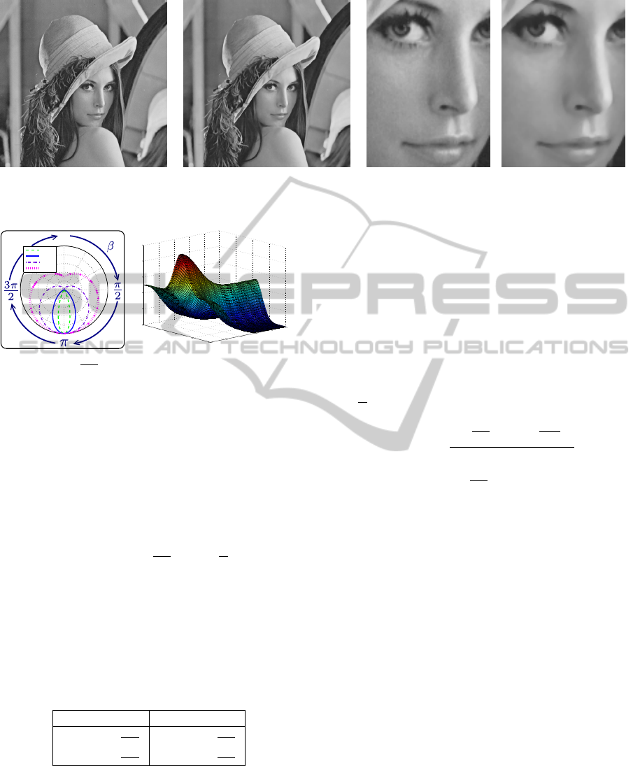
(a) Lena original (b) Our method (c) Enlargement of (a) (d) Enlargement of (b)

Figure 6: Our algorithm applied on a real image polluted by an acquisition noise.

0.2

0.4

0.6

0.8

k = 0.1

k = 0.2

k = 0.5

k = 0.9

0.2

0.4

0.6

0.8

π/2

3π/2

2π

0.2

0.4

0.6

0.8

||∇ I ||

(a) Function e

−



(π−γ)

(π·k)



(b) f

function, k = 0.6

Figure 5: Control functions of the diffusion process.

between θ

and θ

. However, inside homogeneous

regions, due to the level lines on the image surface,

and θ

are not opposite directions (i.e. β 6= π,

see Fig. 6(c)), thus the diffusion does not perform

isotropically. Here, we propose to align the orienta-

tions diffusion when the gradient value is low (i.e.

= θ

+ π). To achieve this, a new angle called γ

between the two edges directions is deﬁned as:

γ = min(β + π ·e

−

k∇Ik

−π ·e

−

,π) (7)

The more k∇Ik is close to zero, the more γ is close

to π (plotted in Fig. 4(a) bottom). The parameter a ∈

]0,1] steers the straightening, as shown in Fig. 4, the

more a is growing, the more γ is close to π for each

pixel. Now, as illustrated in Fig. 4(a), we consider the

two new diffusion directions ρ

and ρ

in our method

(see Section 3.2), estimated modulo 2π in function of

the following table:

> θ

< θ

= θ

γ−β

= θ

−

γ−β

= θ

−

γ−β

= θ

γ−β

3.2 An Approach Preserving Contours

and Smoothing Regions

Our algorithm enables a smoothing in the improved

directions of the contours, thus preserving edges and

details (I

term) while diffusing also in the di-

rection of η for edges having a low gradient or in-

side homogeneous regions (I

ηη

term). Furthermore,

these three directions smoothing terms have to be con-

trolled in order to preserve image contours and not to

create undesired artifacts or ﬁber effect elsewhere. In

this respect, we adapt a new PDE developed in (Mag-

nier and Montesinos, 2013), involving the gradient

magnitude (eq. 5) and the γ angle (eq. 7) driving both

the diffusion terms I

and I

ηη











∂I

∂t

(x,y,t) = f



+ f

·I

ηη



−



k∇Ik



+ e

−



(π−γ)

(π·k)



= e

−



k∇Ik



, with (k, h) ∈]0; 1]

(8)

The f

function ensures the diffusion preserving

edges and corners whereas the f

function enables

a permanent smoothing in the gradient direction for

noisy homogeneous regions. One one hand, the more

the h value is close to 1, the more edges are blurred,

one the other hand the more the k value is close to 1,

the more the diffusion process is important. Contrary

to (Alvarez et al., 1992), these control functions are

not threshold functions but continuous functions (Fig.

5). Thus, the diffusion is never only in the (ρ

,ρ

)

directions. In case of a small gradient and a γ angle

close to π, the considered pixel will be widely dif-

fused (see Fig. 5(a)). If the gradient absolute value is

large and the γ angle is small, smoothing is weak and

operates mainly along these two orientations (ρ

,ρ

4 EXPERIMENTAL RESULTS

AND ANALYSIS

In this section, we present several results of our reg-

ularization method compared to different other PDEs

OrientedHalfGaussianKernelsandAnisotropicDiffusion

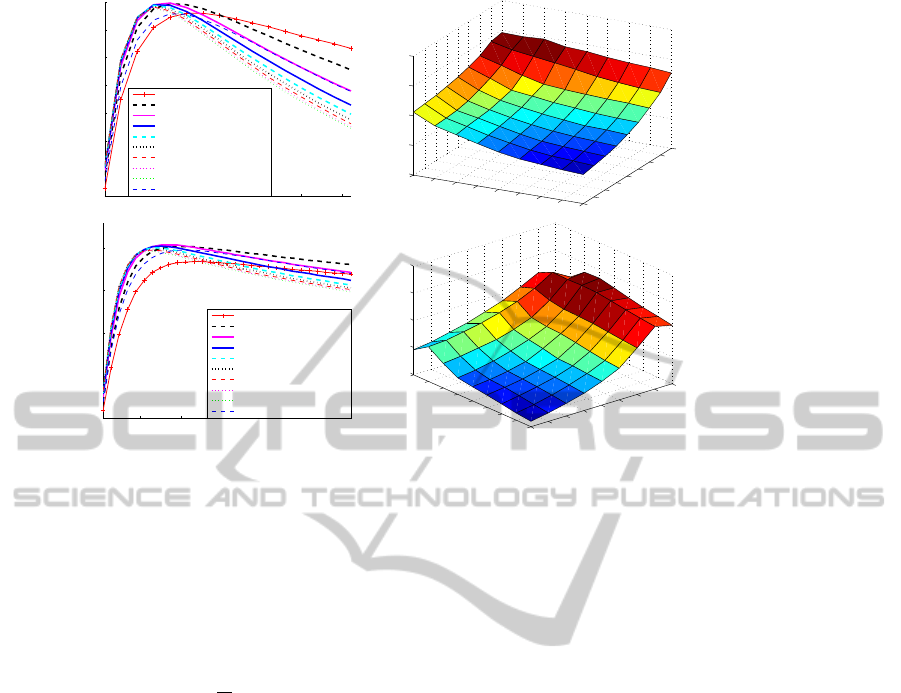
5 10 15 20 25 30

0.72

0.74

0.76

0.78

0.8

0.82

0.84

0.86

Iterations

SSIM

k = 0.1, h = 0.1 and a = 0.1

k = 0.2, h = 0.1 and a = 0.1

k = 0.3, h = 0.1 and a = 0.1

k = 0.4, h = 0.1 and a = 0.1

k = 0.5, h = 0.1 and a = 0.1

k = 0.6, h = 0.1 and a = 0.1

k = 0.7, h = 0.1 and a = 0.1

k = 0.8, h = 0.1 and a = 0.1

k = 0.9, h = 0.1 and a = 0.1

Edges directions, k = 0.3, h = 0.1

0.1

0.2

0.3

0.4

0.5

0.6

0.7

0.8

0.9

0.1

0.2

0.3

0.4

0.5

0.6

0.7

0.8

0.9

0.83

0.84

0.85

0.86

0.87

SSIM

(a) Man image

10 20 30 40 50 60

0.5

0.55

0.6

0.65

0.7

Iterations

SSIM

k = 0.1, h = 0.1 and a = 0.2

k = 0.2, h = 0.1 and a = 0.2

k = 0.3, h = 0.1 and a = 0.2

k = 0.4, h = 0.1 and a = 0.2

k = 0.5, h = 0.1 and a = 0.2

k = 0.6, h = 0.1 and a = 0.2

k = 0.7, h = 0.1 and a = 0.2

k = 0.8, h = 0.1 and a = 0.2

k = 0.9, h = 0.1 and a = 0.2

Edges directions, k = 0.3, h = 0.1

0.1

0.2

0.3

0.4

0.5

0.6

0.7

0.8

0.9

0.1

0.2

0.3

0.4

0.5

0.6

0.7

0.8

0.9

0.68

0.69

0.7

0.71

0.72

SSIM

(b) Barbara image

Figure 7: SSIM evolution in function of the (k,h) parameters. On the right: highest score.

approaches. For each result, presented below, we de-

tail the parameters used either for our algorithm, or

for other methods. Also, we show a SSIM (Wang

et al., 2004) evaluation of noisy images as a function

of the number of iterations using different parameters,

which permits us to discuss about the choice of the

best parameters couple (k,h). Note that, in order to

obtain precise diffusion directions (θ

,θ

), we use a

discretization angle of ∆θ =

= 2

◦

and the standard

deviation of the half anisotropic Gaussian are µ = 5,

λ = 1 for the gradient extraction (eq. 5).

Firstly, the image in Fig. 6(a) is corrupted by

a low acquisition noise because it is a scan of the

original Lena from Playboy. After 10 iterations, our

method removes this noise, and plain regions become

totally homogeneous whereas small objects are well

preserved (see details in Fig. 6(b)). Diffusion parame-

ters are (k,h)=(0.3,0.1) and a = 0.1 because the noise

is low in this image.

The second image shown in Fig. 8(b) is a nat-

ural image contaminated by a Gaussian noise (σ =

10). We aim to regularize this picture and preserve

edges as far as possible. As presented in Fig. 8(g),

(h) and (i), comparing the absolute error between

the original image and the regularized image, our

algorithm preserves better edges than tensorial re-

sults (Tschumperl

e and Deriche, 2005; Tschumperl

2006). To obtain a better visualization, note that the

absolute error images are corrected following a curve

on the image histogram, as presented in Fig. 8(c).

This visualization process is the same for each abso-

lute error image presented in this paper.

The third noisy image presented in Fig. 9(b)

contains a random Gaussian noise of standard devi-

ation σ = 20. Due to this high noise and the tex-

ture, this image is particularly difﬁcult to regularize

correctly while preserving the thin texture. For each

ﬁlter, we choose the parameters that gives the best

results. In order to obtain comparative results, we

choose the same width (i.e. standard deviation) of

the Gaussian kernel for approaches using this function

(i. e. σ = µ = 1 for (Alvarez et al., 1992; Weickert,

1999; Tschumperl

e and Deriche, 2005; Tschumperl

2006)). We compare our result with the MCM (Catt

et al., 1992), the methods of Perona-Malik (Perona

and Malik, 1990), Alvarez et al. (Alvarez et al.,

1992), tensorial driven diffusion (Weickert, 1999;

Tschumperl

e and Deriche, 2005; Tschumperl

e, 2006)

and Magnier et al. (Magnier et al., 2013b).

It is easy to remark that MCM and Perona-Malik

models do not remove correctly the noise. Algorithm

of Alvarez et al. loses the texture and creates arti-

facts at position of edges. Tensors (Weickert, 1999;

Tschumperl

e, 2006) diffusion creates a ﬁber effect in

homogeneous regions due to the high noise. Tenso-

rial result of Tschumperl

e (Tschumperl

e and Deriche,

2005) gives a good result even if this method is known

to distort corners but creates a graininess effect inside

homogeneous regions (see details in Fig. 9(l)). Our

algorithm restores correctly edges (Fig. 9(i)), does not

create undesirable ﬁber effect inside homogeneous re-

gions and enables a regularization of stripes textures

with the use of thin half kernels (details in Fig. 9(m)).

We have tested different values of the couple (k,h)

VISAPP2014-InternationalConferenceonComputerVisionTheoryandApplications

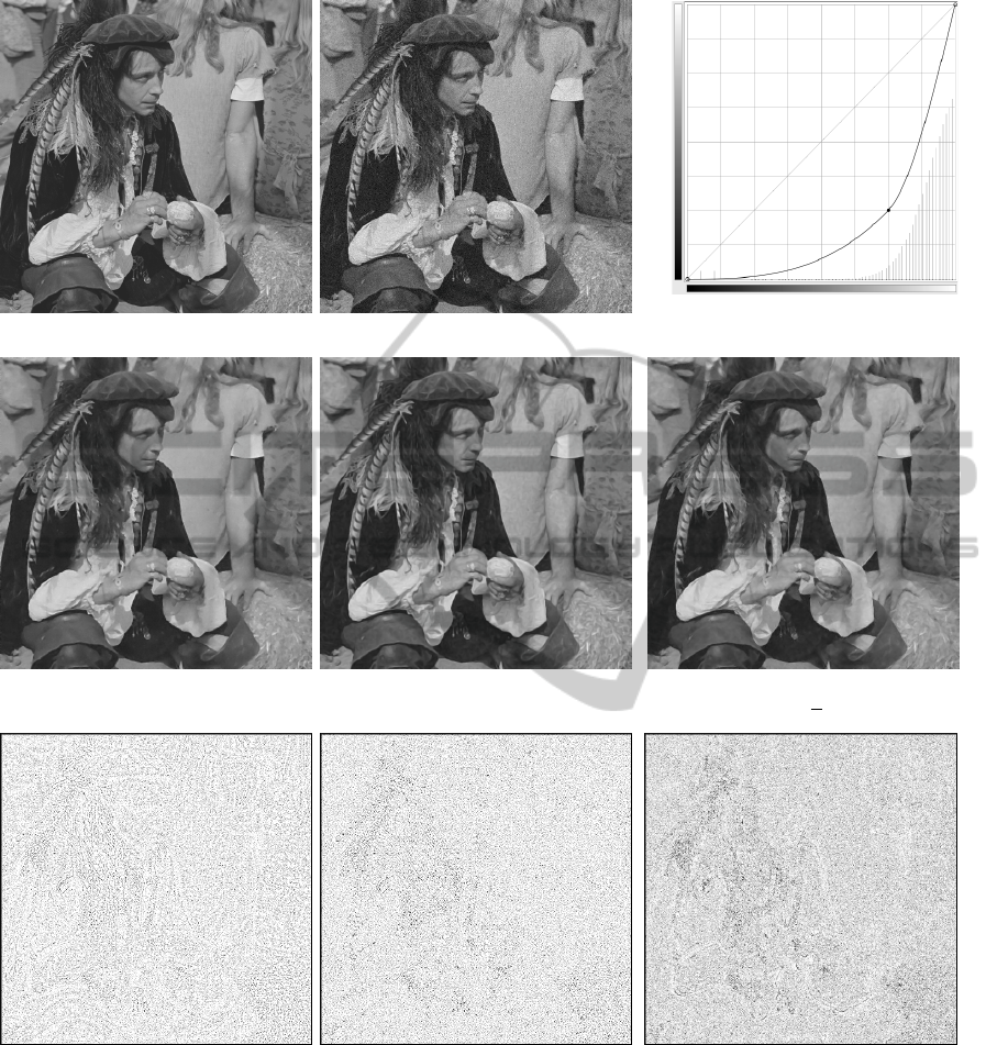
Original error image

Corrected error image

(a) Image of the Man, 512×512 (b) Noisy image, σ = 10 (c) Correction curve of the error

(d) Tensorial result (Tschumperl

e and Deriche, 2005) (e) Tensorial result (Tschumperl

e, 2006) (f) Our result

σ = 1, ρ = 0.7, 20 iterations σ = 1, ρ = 0.7, 20 iterations µ=5, λ=1, ∆θ=

, 12 iterations

(g) Absolute error of (d) (h) Absolute error of (e) (i) Absolute error of (f)

Figure 8: Image regularization and absolute error. Absolute error are negative images.

and when k < h, the diffusion results in blurring

edges. When k 6 0.2, ﬂat regions become totally ho-

mogeneous but the smoothing process is so weak on

edges that they are not retored. Fig. 7 enables a bet-

ter visualization for the choices of the couple (k,h) in

function of the SSIM evolution. It determines that for

(k, h) = (0.3, 0.1), the results are the best with this set

of parameters, only the a parameter (Fig. 4) and the

standard deviations of the half kernels must be set in

function of the image type. Generally, the choice of

our half kernel ﬁlters parameters (µ,λ) has to be done

in function of the noise level. In order to preserve

small objects, we can choose for the length of our ﬁl-

ter µ = 5. However, the width which corresponds to

the derivation ﬁlter depends on the noise level and the

image size. typically, we can choose λ = 1, it enables

to keep precisely edges but if the noise is higher, we

can choose a larger value.

OrientedHalfGaussianKernelsandAnisotropicDiffusion

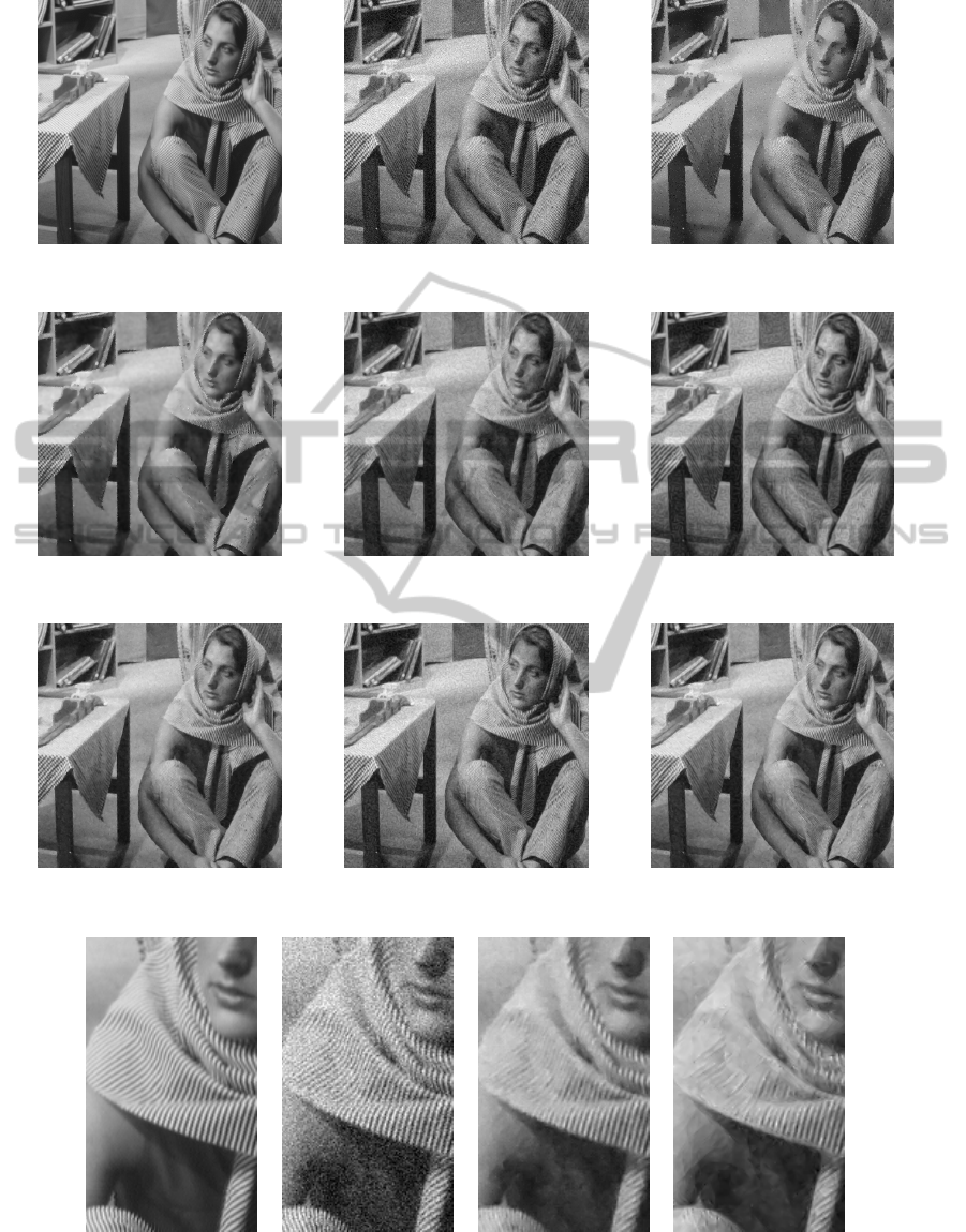
(a) Image of Barbara (b) Degraded image with a (c) Perona-Malik diffusion (Perona and Malik, 1990)

512×512 Gaussian noise: σ = 20 K = 0.05, 100 iterations

(d) Alvarez et al. diffusion (Alvarez et al., 1992) (e) MCM diffusion (Catt

e et al., 1992) (f) Weickert’s result (Weickert, 1999)

σ = 1, 20 iterations, K = 0.02 20 iterations σ = 1, ρ = 0.7, 50 iterations

(g) Tensorial result (Tschumperl

e and Deriche, 2005) (h) Tensorial result (Tschumperl

e, 2006) (i) Our result, k=0.3, h=0.1,

σ = 1, ρ = 0.7, 20 iterations σ = 1, ρ = 0.7, 20 iterations µ=5, λ=1, 20 iterations

(j) Close up in (a) (k) Close up in (b) (l) Close up in (g) (m) Close up in (i)

Figure 9: Enhancement of Barbara image by different PDE methods.

VISAPP2014-InternationalConferenceonComputerVisionTheoryandApplications

5 CONCLUSIONS

In this paper, we have presented a new regulariza-

tion technique based on half Gaussian ﬁltering fol-

lowed by an anisotropic PDE diffusion. This method

complements previous works by calculating new di-

rections of diffusion for a more accurate regulariza-

tion of images. We have shown that the ﬁne assess-

ment of the diffusion direction is a key factor, and

we have proposed a set of control parameters which

provide very good results in restoration of noisy im-

ages. Eventually, as these diffusion directions pre-

serve precisely corners and small objects in images,

future works will focus on the extraction of corners

only using the improved edges directions formula de-

tailed in this paper.

REFERENCES

Alvarez, L., Lions, P.-L., and Morel, J.-M. (1992). Image

selective smoothing and edge detection by nonlinear

diffusion, ii. SIAM J. of Num. Anal., 29(3):845–866.

Aubert, G. and Kornprobst, P. (2006). Mathematical prob-

lems in image processing: partial differential equa-

tions and the calculus of variations (second edition),

volume 147. Springer-Verlag.

Canny, F. (1986). A computational approach to edge detec-

tion. IEEE TPAMI, 8(6):679–698.

Caselles, V. and Morel, J. (1998). Introduction to the special

issue on partial differential equations and geometry-

driven diffusion in image processing and analysis.

IEEE TIP, 7(3):269–273.

Catt

e, F., Lions, P., Morel, J., and Coll, T. (1992). Image

selective smoothing and edge detection by nonlinear

diffusion. SIAM J. of Num. Anal., pages 182–193.

Deriche, R. (1992). Recursively implementing the gaussian

and its derivatives. In ICIP, pages 263–267.

Freeman, W. T. and Adelson, E. H. (1991). The design and

use of steerable ﬁlters. IEEE TPAMI, 13:891–906.

Jacob, M. and Unser, M. (2004). Design of steerable ﬁlters

for feature detection using canny-like criteria. IEEE

TPAMI, 26(8):1007–1019.

Koenderink, J. (1984). The structure of images. Biological

cybernetics, 50(5):363–370.

Kornprobst, P., Deriche, R., and Aubert, G. (1997). Nonlin-

ear operators in image restoration. In ICVPR, pages

325–331.

Magnier, B., Huanyu, X., Montesinos, P., et al. (2013a).

Half gaussian kernels based shock ﬁlter for image de-

blurring and regularization. In VISAPP, volume 1,

pages 51–60.

Magnier, B. and Montesinos, P. (2013). Evolution of im-

age regularization with pdes toward a new anisotropic

smoothing based on half kernels. In IS&T/SPIE

Electronic Imaging, pages 86550M–86550M. Interna-

tional Society for Optics and Photonics.

Magnier, B., Montesinos, P., and Diep, D. (2011a). Fast

Anisotropic Edge Detection Using Gamma Correction

in Color Images. In IEEE 7th ISPA, pages 212–217.

Magnier, B., Montesinos, P., and Diep, D. (2011b). Texture

Removal in Color Images by Anisotropic Diffusion.

In VISAPP, pages 40–50.

Magnier, B., Montesinos, P., and Diep, D. (2012). A new

region-based pde for perceptual image restoration. In

VISAPP, pages 56–65.

Magnier, B., Montesinos, P., Diep, D., et al. (2013b). Per-

ceptual color image smoothing via a new region-based

pde scheme. Electronic Letters on Computer Vision

and Image Analysis 12 (1), 1:17–32.

Michelet, F., Da Costa, J.-P., Lavialle, O., Berthoumieu, Y.,

Baylou, P., and Germain, C. (2007). Estimating local

multiple orientations. Sig. Proc., 87(7):1655–1669.

Montesinos, P. and Magnier, B. (2010). A New Perceptual

Edge Detector in Color Images. In ACIVS, volume 2,

pages 209–220.

uhlich, M., Friedrich, D., and Aach, T. (2012). Design

and implementation of multisteerable matched ﬁlters.

TPAMI, 34(2):279–291.

Perona, P. (1992). Steerable-scalable kernels for edge detec-

tion and junction analysis. IMAVIS, 10(10):663–672.

Perona, P. and Malik, J. (1990). Scale-space and edge

detection using anisotropic diffusion. IEEE TPAMI,

12:629–639.

Simoncelli, E. and Farid, H. (1996). Steerable wedge ﬁlters

for local orientation analysis. IEEE TIP, 5(9):1377–

1382.

Tschumperl

e, D. (2006). Fast anisotropic smoothing

of multi-valued images using curvature-preserving

PDE’s. IJCV, 68(1):65–82.

Tschumperl

e, D. and Deriche, R. (2005). Vector-valued im-

age regularization with pdes: A common framework

for different applications. IEEE TPAMI, pages 506–

517.

Wang, Z., Bovik, A., Sheikh, H., and Simoncelli, E. (2004).

Image quality assessment: From error visibility to

structural similarity. IEEE TIP, 13(4):600–612.

Weickert, J. (1999). Coherence-enhancing diffusion ﬁlter-

ing. IJCV, 31(2):111–127.

OrientedHalfGaussianKernelsandAnisotropicDiffusion