
A Comparative Evaluation of 3D Keypoint Detectors in a RGB-D Object
Dataset
S
´
ılvio Filipe and Lu
´
ıs A. Alexandre
Informatics, IT - Instituto de Telecomunicac¸
˜
oes, University of Beira Interior,
Department of Informatics, 6200-001 Covilh
˜
a, Portugal
Keywords:
3D Keypoints, 3D Interest Points, 3D Object Recognition, Performance Evaluation.
Abstract:
When processing 3D point cloud data, features must be extracted from a small set of points, usually called
keypoints. This is done to avoid the computational complexity required to extract features from all points in a
point cloud. There are many keypoint detectors and this suggests the need of a comparative evaluation. When
the keypoint detectors are applied to 3D objects, the aim is to detect a few salient structures which can be used,
instead of the whole object, for applications like object registration, retrieval and data simplification. In this
paper, we propose to do a description and evaluation of existing keypoint detectors in a public available point
cloud library with real objects and perform a comparative evaluation on 3D point clouds. We evaluate the
invariance of the 3D keypoint detectors according to rotations, scale changes and translations. The evaluation
criteria used are the absolute and the relative repeatability rate. Using these criteria, we evaluate the robustness
of the detectors with respect to changes of point-of-view. In our experiments, the method that achieved better
repeatability rate was the ISS3D method.
1 INTRODUCTION
The computational cost of descriptors is generally
high, so it does not make sense to extract descriptors
from all points in the cloud. Thus, keypoint detec-
tors are used to select interesting points in the cloud
on which descriptors are then computed in these lo-
cations. The purpose of the keypoint detectors is
to determine the points that are different in order to
allow an efficient object description and correspon-
dence with respect to point-of-view variations (Mian
et al., 2010).
This work is motivated by the need to quan-
titatively compare different keypoint detector ap-
proaches, in a common and well established experi-
mentally framework, given the large number of avail-
able keypoint detectors. Inspired by the work on
2D features (Schmid et al., 2000; Mikolajczyk et al.,
2005) and 3D (Salti et al., 2011), and by a similar
work on descriptor evaluation (Alexandre, 2012), a
comparison of several 3D keypoint detectors is made
in this work. In relation to the work of Schmid et al.
(2000); Salti et al. (2011), our novelty is that we use a
real database instead of an artificial, the large number
of 3D point clouds and different keypoint detectors.
Regarding the paper Filipe and Alexandre (2013), the
Input Cloud
Transformation
Keypoint
Detector
Inverse
Transformation
Keypoints
Correspondence
Keypoint
Detector
Figure 1: Keypoint detectors evaluation pipeline used in this
paper.
current paper introduces in the evaluation of 4 new
keypoint detectors, makes a computational complex-
ity evaluation through the time spent by each method
on the experiments. The benefit of using real 3D point
clouds is that it reflects what happens in real life, such
as, with robot vision. These never “see” a perfect or
complete object, like the ones present by artificial ob-
jects.
The keypoint detectors evaluation pipeline used in
this paper is presented in figure 1. To evaluate the
invariance of keypoint detection methods, we extract
the keypoints directly from the original cloud. More-
over, we apply a transformation to the original 3D
point cloud before extracting another set of keypoints.
Once we get these keypoints from the transformed
cloud, we apply an inverse transformation, so that we
can compare these with the keypoints extracted from
the original cloud. If a particular method is invari-
ant to the applied transformation, the keypoints ex-
476
Filipe S. and A. Alexandre L..
A Comparative Evaluation of 3D Keypoint Detectors in a RGB-D Object Dataset.
DOI: 10.5220/0004679904760483
In Proceedings of the 9th International Conference on Computer Vision Theory and Applications (VISAPP-2014), pages 476-483
ISBN: 978-989-758-003-1
Copyright
c
2014 SCITEPRESS (Science and Technology Publications, Lda.)

tracted directly from the original cloud should corre-
spond to the keypoints extracted from the cloud where
the transformation was applied.
The low price of 3D cameras has increased expo-
nentially and the interest in using depth information
for solving vision tasks. A useful resource for users of
this type of sensors is the Point Cloud Library (PCL)
(Rusu and Cousins, 2011) which contains many al-
gorithms that deal with point cloud data, from seg-
mentation to recognition, from search to input/output.
This library is used to deal with real 3D data and we
used it to evaluate the robustness of the detectors with
variations of the point-of-view in real 3D data.
The organization of this paper is as follows: the
next section presents a detailed description of the
methods that we evaluate; the results and the discus-
sion appear in section 3; and finally, we end the paper
in section 4 with the conclusions.
2 EVALUATED 3D KEYPOINT
DETECTORS
Our goal was to evaluate the available descriptors
in the current PCL version (1.7 pre-release, on June
2013).
There are some keypoint detectors in PCL which
we will not consider in this paper, since they are not
applicable to point cloud data directly or only sup-
port 2D point clouds. These are: Normal Aligned Ra-
dial Feature (NARF) (Steder et al., 2010) that assume
the data to be represented by a range image (2D im-
age showing the distance to points in a scene from a
specific point); AGAST (Mair et al., 2010) and Bi-
nary Robust Invariant Scalable Keypoints (BRISK)
(Leutenegger et al., 2011) that only support 2D point
clouds.
2.1 Harris3D
The Harris method (Harris and Stephens, 1988) is
a corner and edge based method and these types
of methods are characterized by their high-intensity
changes in the horizontal and vertical directions.
These features can be used in shape and motion
analysis and they can be detected directly from the
grayscale images. For the 3D case, the adjustment
made in PCL for the Harris3D detector replaces the
image gradients by surface normals. With that, they
calculate the covariance matrix Cov around each point
in a 3×3 neighborhood. The keypoints response mea-
sured at each pixel coordinates (x,y,z) is then defined
by
r(x, y,z) = det(Cov(x,y, z)) −k (trace(Cov(x,y,z)))
2
,
(1)
where k is a positive real valued parameter. This pa-
rameter serves roughly as a lower bound for the ratio
between the magnitude of the weaker edge and that of
the stronger edge.
To prevent too many keypoints from lumping to-
gether closely, a non-maximal suppression process on
the keypoints response image is usually carried out
to suppress weak keypoints around the stronger ones,
followed by a thresholding process.
2.2 Harris3D Variants
In the PCL, we can find two variants of the Harris3D
keypoint detector: these are called Lowe and Noble.
The differences between them are the functions that
define the keypoints response (equation 1). Thus, for
the Lowe method the keypoints response is given by:
r(x, y,z) =
det(Cov(x,y,z))
trace(Cov(x,y,z))
2
. (2)
The keypoints response from Noble method is
given by:
r(x, y,z) =
det(Cov(x,y,z))
trace(Cov(x,y,z))
. (3)
2.3 Kanade-Lucas-Tomasi
The Kanade-Lucas-Tomasi (KLT) detector (Tomasi
and Kanade, 1991) was proposed a few years after
the Harris detector. In the 3D version presented in
the PCL, this keypoint detector has the same basis as
the Harris3D detector. The main differences are: the
covariance matrix is calculated directly in the input
value instead of the normal surface; and for the key-
points response they used the first eigen value of the
covariance matrix around each point in a 3 ×3 neigh-
borhood. The suppression process was similar to the
one used in the Harris3D method. In this method,
they remove the smallest eigen values by threshold-
ing these ones.
2.4 Curvature
Surface curvature has been used extensively in the lit-
erature for cloud simplification and smoothing (Des-
brun et al., 1999), object recognition (Yamany and
Farag, 2002) and segmentation (Jagannathan and
Miller, 2007). However, there is a lack of a sys-
tematic approach in extracting salient local features
or keypoints from an input surface normals using its
AComparativeEvaluationof3DKeypointDetectorsinaRGB-DObjectDataset
477

local curvature information at multiple scales. The
curvature method in PCL calculates the principal sur-
face curvatures on each point using the surface nor-
mals. The keypoints response image is used to sup-
press weak keypoints around the stronger ones and
such a process is the same as performed in the me-
thod of Harris3D.
2.5 SIFT3D
The Scale Invariant Feature Transform (SIFT) key-
point detector was proposed by Lowe (2001). The
SIFT features are represented by vectors that repre-
sent local cloud measurements. The main steps used
by the SIFT detector when locating keypoints are pre-
sented below.
The original algorithm for 3D data was presented
by Flint et al. (2007), which uses a 3D version of the
Hessian to select such interest points. A density func-
tion f (x,y, z) is approximated by sampling the data
regularly in space. A scale space is built over the den-
sity function, and a search is made for local maxima
of the Hessian determinant.
The input cloud, I(x, y, z) is convolved with a
number of Gaussian filters whose standard deviations
{σ
1
,σ
2
,...} differ by a fixed scale factor. That is,
σ
j+1
= kσ
j
where k is a constant scalar that should be
set to
√
2. The convolutions yield smoothed images,
denoted by
G(x,y,z,σ
j
),i = 1,..., n. (4)
The adjacent smoothed images are then subtracted
to yield a small number (3 or 4) of Difference-of-
Gaussian (DoG) clouds, by
D(x,y,z,σ
j
) = G(x,y, z, σ
j+1
) −G(x, y, z, σ
j
). (5)
These two steps are repeated, yielding a number
of DoG clouds over the scale space.
Once DoG clouds have been obtained, keypoints
are identified as local minima/maxima of the DoG
clouds across scales. This is done by comparing
each point in the DoG clouds to its eight neighbors at
the same scale and nine corresponding neighborhood
points in each of the neighborhood scales. If the point
value is the maximum or minimum among all com-
pared points, it is selected as a candidate keypoint.
The keypoints identified from the above steps are
then examined for possible elimination if the two lo-
cal principal curvatures of the intensity profile around
the keypoint exceed a specified threshold value. This
elimination step involves estimating the ratio between
the some eigenvalues of the Hessian matrix (i.e., the
second partial derivatives) of the local cloud intensity
around each keypoint.
2.6 SUSAN
The Smallest Univalue Segment Assimilating Nu-
cleus (SUSAN) corner detector has been introduced
by Smith and Brady (1997). Many corner detectors
using various criteria for determining “cornerness” of
image points are described in the literature (Smith and
Brady, 1997). SUSAN is a generic low-level image
processing technique, which apart from corner detec-
tion has also been used for edge detection and noise
suppression.
The significance of the thresholding step with the
fixed value g =
n
max
2
(geometric threshold) is simply
a precise restatement of the SUSAN principle: if the
nucleus lies on a corner then the Univalue Segment
Assimilating Nucleus (USAN) area will be less than
half of its possible value, n
max
. USAN is a mea-
sure of how similar a center pixel’s intensity is to
those in its neighborhood. The gray value similar-
ity function s(g
1
,g
2
) measures the similarity between
the gray values g
1
and g
2
. s is meant to be similar in
shape to a step function
X
t
: [0, 255]
2
−→ [0,1]
(g
1
,g2) 7−→
1 i f |g
1
−g
2
| ≤ t
0 otherwise
(6)
where t ∈ [1,256] is the brightness difference thresh-
old value. Summing over this kind of function for a
set of pixels is equivalent to counting the number of
similar pixels, i.e., pixels whose gray value difference
is at most t. It can be used to adjust the detector’s
sensitivity to the image’s global contrast level.
SUSAN uses the smooth gray value similarity
function
s
t
: [0, 255]
2
−→ [0,1]
(g
1
,g2) 7−→ e
−
g
1
−g
2
t
(7)
which is mentioned to perform better than the step
function X
t
. The smoothness of s
t
plays an important
role in noise suppression (Smith and Brady, 1997),
since s
t
only depends on the difference between g
1
and g
2
.
To make the method more robust, points closer
in value to the nucleus receive a higher weighting.
Moreover, a set of rules presented in Smith (1992) are
used to suppress qualitatively “bad” keypoints. Lo-
cal minima of the SUSANs are then selected from the
remaining candidates.
2.7 ISS3D
Intrinsic Shape Signatures (ISS) (Zhong, 2009) is a
method relying on region-wise quality measurements.
VISAPP2014-InternationalConferenceonComputerVisionTheoryandApplications
478
This method uses the magnitude of the smallest eigen-
value (to include only points with large variations
along each principal direction) and the ratio between
two successive eigenvalues (to exclude points having
similar spread along principal directions).
The ISS S
i
= {F
i
, f
i
} at a point p
i
consists of two
components: 1 – The intrinsic reference frame F
i
=
{p
i
,{e
x
i
,e
y
i
,e
z
i
}}where p
i
is the origin, and {e
x
i
,e
y
i
,e
z
i
}
is the set of basis vectors. The intrinsic frame is a
characteristic of the local object shape and indepen-
dent of viewpoint. Therefore, the view independent
shape features can be computed using the frame as a
reference. However, its basis {e
x
i
,e
y
i
,e
z
i
}, which spec-
ifies the vectors of its axes in the sensor coordinate
system, are view dependent and directly encode the
pose transform between the sensor coordinate system
and the local object-oriented intrinsic frame, thus en-
abling fast pose calculation and view registration. 2 –
The 3D shape feature vector f
i
= ( f
i0
, f
i1
,..., f
iK−1
),
which is a view independent representation of the
local/semi-local 3D shape. These features can be
compared directly to facilitate the matching of surface
patches or local shapes from different objects.
Only points whose ratio between two succes-
sive eigenvalues is below a threshold are considered.
Among these points, the keypoints are given by the
magnitude of the smallest eigenvalue, so as to con-
sider as keypoints only those points exhibiting a large
variation along every principal direction.
3 EXPERIMENTAL EVALUATION
AND DISCUSSION
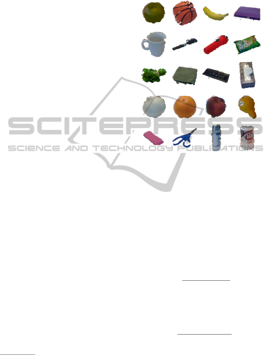
3.1 Dataset
To perform the evaluation of keypoint detectors, we
use the large RGB-D Object Dataset
1
(Lai et al.,
2011). This dataset is a hierarchical multi-view ob-
ject dataset collected using an RGB-D camera. The
dataset contains clouds of 300 physically distinct ob-
jects taken from multiple views, organized into 51
categories, containing a total of 207621 segmented
clouds. Examples of some objects are shown in fig-
ure 2. The chosen objects are commonly found in
home and office environments, where personal robots
are expected to operate.
3.2 Keypoints Correspondence
The correspondence between the keypoints extracted
1
The dataset is publicly available at http://www.cs.
washington.edu/rgbd-dataset.
Figure 2: Examples of some objects of the RGB-D Object
Dataset.
directly from the original cloud and the ones extracted
from transformed cloud is done using the 3D point-
line distance (Weisstein, 2005). A line in three dimen-
sions can be specified by two points p
1
= (x
1
,y
1
,z
1
)
and p
2
= (x
2
,y
2
,z
2
) lying on it, then a vector line is
produced. The squared distance between a point on
the line with parameter t and a point p
0
= (x
0
,y
0
,z
0
)
is therefore
d
2
= [(x
1
−x
0
) + (x
2
−x
1
)t]
2
+ [(y
1
−y
0
)+
(y
2
−y
1
)t]
2
+ [(z
1
−z
0
) + (z
2
−z
1
)t]
2
.
(8)
To minimize the distance, set ∂(d
2
)/∂t = 0 and solve
for t to obtain
t = −
(p
1
−p
0
) ·(p
2
−p
1
)
|p
2
−p
1
|
2
, (9)
where · denotes the dot product. The minimum dis-
tance can then be found by plugging t back into equa-
tion 8. Using the vector quadruple product ((A ×
B)
2
= A
2
B
2
−(A ·B)
2
) and taking the square root re-
sults, we can obtain:
d =
|(p
0
−p
1
) ×(p
0
−p
2
)|
|p
2
−p
1
|
, (10)
where × denotes the cross product. Here, the numer-
ator is simply twice the area of the triangle formed
by points p
0
, p
1
, and p
2
, and the denominator is the
length of one of the bases of the triangle.
AComparativeEvaluationof3DKeypointDetectorsinaRGB-DObjectDataset
479

3.3 Measures
The most important feature of a keypoint detector is
its repeatability. This feature takes into account the
capacity of the detector to find the same set of key-
points in different instances of a particular model. The
differences may be due to noise, view-point change,
occlusion or by a combination of the above.
The repeatability measure used in this paper is ba-
sed on the measure used in (Schmid et al., 2000) for
2D keypoints and in (Salti et al., 2011) for 3D key-
points. A keypoint extracted from the model M
h
, k
i
h
transformed according to the rotation, translation or
scale change, (R
hl
,t
hl
), is said to be repeatable if the
distance d (given by the equation 10) from its nearest
neighbor, k
j
l
, in the set of keypoints extracted from the
scene S
l
is less than a threshold ε, d < ε.
We evaluate the overall repeatability of a detector
both in relative and absolute terms. Given the set RK
hl
of repeatable keypoints for an experiment involving
the model-scene pair (M
h
,S
l
), the absolute repeatabil-
ity is defined as
r
abs
= |RK
hl
| (11)
and the relative repeatability is given by
r =
|RK
hl
|
|K
hl
|
. (12)
The set K
hl
is the set of all the keypoints extracted
on the model M
h
that are not occluded in the scene
S
l
. This set is estimated by aligning the keypoints
extracted on M
h
according to the rotation, transla-
tion and scale and then checking for the presence of
keypoints in S
l
in a small neighborhood of the trans-
formed keypoints. If at least a keypoint is present
in the scene in such a neighborhood, the keypoint is
added to K
hl
.
3.4 Results and Discussion
In this article, we intend to evaluate the invariance of
the methods presented, in relation to rotation, transla-
tion and scale changes. For this, we vary the rotation
according to the three axes (X, Y and Z). The rotations
applied ranged from 5
o
to 45
o
, with 10
o
step. The
translation is performed simultaneously in the three
axes and the image displacement applied on each axis
is obtained randomly. Finally, we apply random vari-
ations (between ]1×,5×]) to the scale.
In table 1, we present some results about each
keypoint detector applied to the original clouds. The
percentage of clouds where the keypoint detectors
successfully extracted (more than one keypoint) is
Table 1: Statistics about each keypoint detector. These val-
ues come from processing the original clouds.
Keypoint % Keypoint
Mean of
Mean
detectors clouds
extracted
time (s)
keypoints
Harris3D 99.99 85.63 1.05
SIFT3D 99.68 87.46 9.54
ISS3D 97.97 86.24 1.07
SUSAN 86.51 242.38 1.64
Lowe 99.99 85.12 1.02
KLT 100.00 99.16 1.03
Curvature 99.96 119.36 0.70
Noble 99.99 85.12 1.04
presented in column 2. In the column 3, it ap-
pears the mean number of keypoints extracted by
cloud. And finally, we present the mean computa-
tion time (in seconds) spent by each method to ex-
tract the keypoints. These times were obtained on
a computer with Intel
R
Core
TM
i7-980X Extreme Edi-
tion 3.33GHz with 24 GB of RAM memory.
To make a fair comparison between the descrip-
tors, all steps in the pipeline (see figure 1) are equal.
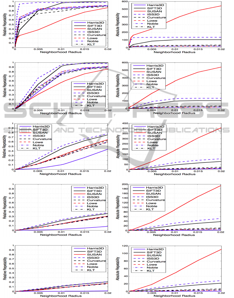
Figures 3 and 4 show the results of the evaluation of
the different methods with various applied transfor-
mations. The threshold distances (ε) analyzed vary
between [0, 2] cm, with small jumps in a total of 33
equally spaced distances calculated. As we saw in
section 2, the methods have a relatively large set of
parameters to be adjusted: the values used were the
ones set by default in PCL.
Regarding the relative repeatability (shown in fig-
ures 3(a), 3(c), 3(e), 3(g), 3(i), 4(a) and 4(c)) the
methods presented have a fairly good performance in
general. In relation to the rotation (see figures 3(a),
3(c), 3(e), 3(g) and 3(i)), increasing the rotation an-
gle of the methods tends to worsen the results. Ide-
ally, the method results should not change indepen-
dently of the transformations applied. Regarding the
applied rotation, the method ISS3D is the one that
provides the best results. In this transformation (ro-
tation), the biggest difference that appears between
the various methods is in the 5 degrees rotation. In
this case, the method ISS3D achieves almost total cor-
respondence keypoints with a distance between them
of 0.25 cm. Whereas for example the SIFT3D only
achieves this performance for keypoints at a distance
of 1 cm. In both the scaling and translation (shown in
figures 4(a) and 4(c)), the methods exhibit very sim-
ilar results to those obtained for small rotations (5
o
rotation in figure 3(a)) with the exception of the SU-
SAN method, that has a relatively higher invariance
to scale changes.
Figures 3(b), 3(d), 3(f), 3(h), 3(i), 4(b) and 4(d)
VISAPP2014-InternationalConferenceonComputerVisionTheoryandApplications
480
(a) Relative repeatability for 5
o
rotation. (b) Absolute repeatability for 5
o
rotation.
(c) Relative repeatability for 15
o
rotation. (d) Absolute repeatability for 15
o
rotation.
(e) Relative repeatability for 25
o
rotation. (f) Absolute repeatability for 25
o
rotation.
(g) Relative repeatability for 35
o
rotation. (h) Absolute repeatability for 35
o
rotation.
(i) Relative repeatability for 45
o
rotation. (j) Absolute repeatability for 45
o
rotation.
Figure 3: Rotation results represented by the relative and absolute repeatability measures (best viewed in color). The relative
repeatability is presented in figures (a), (c), (e), (g) and (i), and the absolute repeatability in figures (b), (d), (f), (h) and (j).
The presented neighborhood radius is in meters.
AComparativeEvaluationof3DKeypointDetectorsinaRGB-DObjectDataset
481
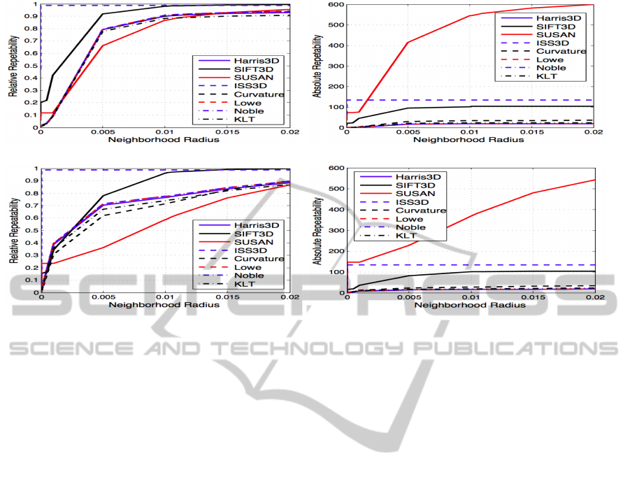
(a) Relative repeatability for scale change. (b) Absolute repeatability for scale change.
(c) Relative repeatability for translation cloud. (d) Absolute repeatability for translation cloud.
Figure 4: Relative and absolute repeatability measures for the scale change and translation clouds (best viewed in color). The
relative repeatability is presented in figures (a) and (c), and the absolute repeatability in figures (b) and (d). The presented
neighborhood radius is in meters.
show the absolute repeatability, that present the num-
ber of keypoints obtained by the methods. With these
results we can see that the method that has higher
absolute repeatability (SUSAN) is not the one that
shows the best performance in terms of relative re-
peatability. In terms of the absolute repeatability,
the ISS3D and SIFT3D have better results than the
SUSAN method regarding the invariance transforma-
tions evaluated in this work.
4 CONCLUSIONS
In this paper, we focused on the available keypoint
detectors on the PCL library, explaining how they
work, and made a comparative evaluation on public
available data with real 3D objects. The experimen-
tal comparison proposed in this work has outlined as-
pects of state-of-the-art methods for 3D keypoint de-
tectors. This work allowed us to evaluate the best per-
formance in terms of various transformations (rota-
tion, scaling and translation).
The novelty of our work compared with the work
of Schmid et al. (2000) and Salti et al. (2011) is: we
are using a real database instead of an artificial, the
large number of point clouds and different keypoint
detectors. The benefit of using a real database is that
our objects have “occlusion”. This type of “occlu-
sion” is made by some kind of failure in the infrared
sensor of the camera or from the segmentation me-
thod. In artificial objects this does not happen, so the
keypoint methods may have better results, but our ex-
periments reflect what can happen in real life, such as,
with robot vision.
Overall, SIFT3D and ISS3D yielded the best
scores in terms of repeatability and ISS3D demon-
strated to be the more invariant. Future work includes
extension of some methodologies proposed for the
keypoint detectors to work with large rotations and
occlusions, and the evaluation of the best combina-
tion of keypoint detectors/descriptors.
ACKNOWLEDGEMENTS
This work is supported by ‘FCT - Fundac¸
˜
ao para a
Ci
ˆ
encia e Tecnologia’ (Portugal) through the research
grant ‘SFRH/BD/72575/2010’, and the funding from
‘FEDER - QREN - Type 4.1 - Formac¸
˜
ao Avanc¸ada’,
subsidized by the European Social Fund and by Por-
tuguese funds through ‘MCTES’.
We also acknowledge the support given by the
IT - Instituto de Telecomunicac¸
˜
oes through ‘PEst-
OE/EEI/LA0008/2013’.
REFERENCES
Alexandre, L. A. (2012). 3D descriptors for object and cate-
gory recognition: a comparative evaluation. In Work-
VISAPP2014-InternationalConferenceonComputerVisionTheoryandApplications
482

shop on Color-Depth Camera Fusion in Robotics at
the IEEE/RSJ International Conference on Intelligent
Robots and Systems (IROS), Vilamoura, Portugal.
Desbrun, M., Meyer, M., Schr
¨
oder, P., and Barr, A. H.
(1999). Implicit fairing of irregular meshes using dif-
fusion and curvature flow. In Proceedings of the 26th
annual conference on Computer graphics and inter-
active techniques, pages 317–324, New York, USA.
Filipe, S. and Alexandre, L. A. (2013). A Comparative
Evaluation of 3D Keypoint Detectors. In 9th Con-
ference on Telecommunications, Conftele 2013, pages
145–148, Castelo Branco, Portugal.
Flint, A., Dick, A., and Hengel, A. (2007). Thrift: Local 3D
Structure Recognition. In 9th Biennial Conference of
the Australian Pattern Recognition Society on Digital
Image Computing Techniques and Applications, pages
182–188.
Harris, C. and Stephens, M. (1988). A combined corner
and edge detector. In Alvey Vision Conference, pages
147–152, Manchester.
Jagannathan, A. and Miller, E. L. (2007). Three-
dimensional surface mesh segmentation using
curvedness-based region growing approach. IEEE
Transactions on Pattern Analysis and Machine
Intelligence, 29(12):2195–2204.
Lai, K., Bo, L., Ren, X., and Fox, D. (2011). A large-scale
hierarchical multi-view RGB-D object dataset. In In-
ternational Conference on Robotics and Automation,
pages 1817–1824.
Leutenegger, S., Chli, M., and Siegwart, R. Y. (2011).
BRISK: Binary Robust invariant scalable keypoints.
In International Conference on Computer Vision,
pages 2548–2555.
Lowe, D. (2001). Local feature view clustering for 3D ob-
ject recognition. Computer Vision and Pattern Recog-
nition, 1:I–682–I–688.
Mair, E., Hager, G., Burschka, D., Suppa, M., and
Hirzinger, G. (2010). Adaptive and Generic Corner
Detection Based on the Accelerated Segment Test.
In European Conference on Computer Vision, pages
183–196.
Mian, A., Bennamoun, M., and Owens, R. (2010). On
the Repeatability and Quality of Keypoints for Lo-
cal Feature-based 3D Object Retrieval from Cluttered
Scenes. International Journal of Computer Vision,
89(2-3):348–361.
Mikolajczyk, K., Tuytelaars, T., Schmid, C., Zisserman, A.,
Matas, J., Schaffalitzky, F., Kadir, T., and Gool, L. V.
(2005). A Comparison of Affine Region Detectors. In-
ternational Journal of Computer Vision, 65(1-2):43–
72.
Rusu, R. B. and Cousins, S. (2011). 3D is here: Point
Cloud Library (PCL). In International Conference on
Robotics and Automation, Shanghai, China.
Salti, S., Tombari, F., and Stefano, L. D. (2011). A Perfor-
mance Evaluation of 3D Keypoint Detectors. In Inter-
national Conference on 3D Imaging, Modeling, Pro-
cessing, Visualization and Transmission, pages 236–
243.
Schmid, C., Mohr, R., and Bauckhage, C. (2000). Evalua-
tion of Interest Point Detectors. International Journal
of Computer Vision, 37(2):151–172.
Smith, S. M. (1992). Feature based image sequence under-
standing.
Smith, S. M. and Brady, J. M. (1997). SUSAN – A new
approach to low level image processing. International
Journal of Computer Vision, 23(1):45–78.
Steder, B., Rusu, R. B., Konolige, K., and Burgard, W.
(2010). NARF: 3D range image features for object
recognition. In Intelligent Robots and Systems, Taipei,
Taiwan.
Tomasi, C. and Kanade, T. (1991). Detection and Tracking
of Point Features. Technical report, Carnegie Mellon
University.
Weisstein, E. W. (2005). The CRC Encyclopedia of Mathe-
matics. CRC Press, 3rd edition.
Yamany, S. M. and Farag, A. A. (2002). Surface signa-
tures: an orientation independent free-form surface
representation scheme for the purpose of objects reg-
istration and matching. IEEE Transactions on Pattern
Analysis and Machine Intelligence, 24(8):1105–1120.
Zhong, Y. (2009). Intrinsic shape signatures: A shape de-
scriptor for 3D object recognition. International Con-
ference on Computer Vision Workshops, pages 689–
696.
AComparativeEvaluationof3DKeypointDetectorsinaRGB-DObjectDataset
483
