
Segmentation of Optic Disc in Retina Images using Texture
Suraya Mohammad
1
, D. T. Morris
1
and Neil Thacker
2
1
School of Computer Science, University of Manchester, Kilburn Building, Oxford Road, Manchester, U.K.
2
ISBE, Medical School, University of Manchester, Stop ford Building, Oxford Road, Manchester, U.K.
Keywords:
Optic Disc Segmentation, BRIEF, Texture.
Abstract:
The paper describes our work on the segmentation of the optic disc in retinal images. Our approach comprises
of two main steps; a pixel classification method to identify pixels that may belong to the optic disc boundary
and a circular template matching method to estimate the circular approximation of the optic disc boundary.
The features used are based on texture, calculated using the intensity differences of local image patches. This
was adapted from Binary Robust Independent Elementary Features (BRIEF). BRIEF is inherently invariant
to image illumination and has a lower degree of computational complexity compared to other existing texture
measurement methods. Fuzzy C-Means (FCM) and Naive Bayes are the clustering and classifier used to
cluster/classify the image pixels. The method was tested on a set of 196 images composed of 110 healthy
retina images and 86 glaucomatous images. The average mean overlap ratio between the true optic disc region
and segmented region is 0.81 for both FCM and Naive Bayes. Comparison with a method based on the Hough
Transform is also provided.
1 INTRODUCTION
The evaluation of retinal images is a diagnostic tool
widely used to gather important clinical information,
such as for diabetic retinopathy and glaucoma assess-
ment, due to its noninvasive nature. These diseases
are two of the main cause of visual impairment world-
wide (Congdon et al., 2003). Both are asymptomatic
in nature, therefore early detection is vital to prevent
complete visual loss. Segmentation of the optic disc
represents the starting point of many automatic com-
puter based methods used to assist the ophthalmolo-
gist in detecting these two diseases.
The Cup-to-Disc (CDR) ratio is commonly used
clinically to asses glaucoma progression. CDR is ob-
tained by measuring the ratio between the vertical di-
ameter of the optic disc cup and the optic disc rim. As
for diabetic retinopathy assessment, the identification
of the optic disc is important to reduce misclassifica-
tion in the automatic detection of other lesions.
Some of the difficulties experienced in the seg-
mentation of the optic disc may be appreciated by Fig-
ure 1 which shows an image of a healthy retina (Fig-
ure 1(a)) and a glaucomatous retina (Figure 1(b)). On
a healthy retina, the optic disc appears as bright and
yellowish, normally with a circular or slightly ellip-
tical shape. However these features and its size may
vary between images. The contrast around the optic
disc boundary is also not constant, normally brighter
(a) (b)
Figure 1: Healthy and glaucomatous retina images.
on the temporal side and less so on the nasal side.
In addition, part of the optic disc boundary may be
obscured by the outgoing blood vessels. Sometimes
there exist bright regions near the edge of the disc
caused by peripapillary atrophy (Figure 1(b)). This
is more common in glaucomatous images compared
to normal images. Retinal images also suffer from
non uniform illumination due to how the image is cap-
tured. This non-uniform illumination results in shad-
ing artefacts and vignetting (Hoover and Goldbaum,
2003), hindering both quantitative image analysis and
the reliable operation of subsequent global operators
(Winder et al., 2009).
In this paper we present an automated segmenta-
tion of the optic disc combining pixel classification
and circular template matching. We used texture fea-
tures based on Binary Robust Independent Elemen-
tary Feature (BRIEF) (Calonder et al., 2010) to clas-
293
Mohammad S., T. Morris D. and Thacker N..
Segmentation of Optic Disc in Retina Images using Texture.
DOI: 10.5220/0004680802930300
In Proceedings of the 9th International Conference on Computer Vision Theory and Applications (VISAPP-2014), pages 293-300
ISBN: 978-989-758-003-1
Copyright
c
2014 SCITEPRESS (Science and Technology Publications, Lda.)

sify the image pixels. BRIEF is inherently invariant
to image illumination, which in our opinion will han-
dle the illumination issue faced by the retinal images.
It is also has a lower degree of computational com-
plexity compared other texture measurements. Naive
Bayes and Fuzzy C Means (FCM) are used as the clas-
sifier and the clustering method respectively to clas-
sify/cluster the image pixels. To obtain the final circu-
lar approximation of the optic disc circular template
matching is used. This is to approximate the optic
disc boundary in the case of (1) not all of the optic disc
boundary is detected and (2) there exist large gaps due
to vessel passing in and out of the eye.
We validate our result with a retina image data
set consisting of both normal and glaucomatous im-
ages. We also compare our result with another
commonly known template matching approach, the
Hough Transform.
2 LITERATURE REVIEW
A number of studies have reported work on optic disc
segmentation. Among the existing techniques, the de-
formable or active contour (snake) has been used in
(Joshi et al., 2011; Lowell et al., 2004; Morris and
Donnison, 1999; Muramatsu et al., 2011). The main
advantage of using this approach is the ability to ob-
tain an accurate optic disc boundary. This is possible
because the active contour has the ability to change
shape depending on the properties of the image, de-
sired contour properties and/or knowledge based con-
straints (Kass et al., 1988). There are two types of
active contour currently used for optic disc segmen-
tation, region based active contour or gradient-based
active contour.
The gradient based active contour normally relies
on the image gradient or edges to influence the en-
ergy forces to evolve to the true optic disc bound-
ary. The presence of the blood vessels, atrophy, low
contrast optic disc boundary and strong optic cup
boundary may prevent the snake from evolving to the
true optic disc boundary. Thus several preprocessing
steps are often implemented prior to snake implemen-
tation, such as by performing blood vessel removal
through morphological filtering as in (May, 2008) or
histogram equalisation followed by thresholding and
pyramid edge detection to enhance the edge (Morris
and Donnison, 1999).
Region based active contour models on the other
hand make use of statistical information from the
background and foreground regions to minimise the
energy function to best separate the regions (Joshi
et al., 2011). The region based active contour is more
robust against local gradient variations. However in
the case where the object to be segmented and the
background regions are heterogeneous and have simi-
lar statistical model, erroneous segmentation may oc-
cur. Thus additional information such as local infor-
mation from multiple image channels is used in (Joshi
et al., 2011).
Another technique used for optic disc segmenta-
tion is circular and elliptical template matching. The
Hough Transform is one of the commonest circular
and elliptical template matching techniques used for
optic disc segmentation. The matching is performed
on an edge map extracted from the underlying image.
The optic disc boundary found through this method is
an approximation and may be not as precise as that
obtained from deformable contour. One main advan-
tage of the Hough Transform technique is that it is
relatively unaffected by noise and gaps in the edge
feature (Lowell et al., 2004). Thus it is very useful
when attempting to determine the optic disc contour
which has no clearly defined edges and is broken by
ingoing and outgoing blood vessels. However obtain-
ing good edge descriptors is vital for the success of
the Hough transform. Otherwise unacceptable results
may be given such as hitting either the curved blood
vessel segments or the strong cup boundary (Lowell
et al., 2004).
Recently pixel classification has been used to seg-
ment the optic disc. Pixel classification is where ev-
ery pixel in the retina image will be classified into a
class, such as optic disc or background. In (Mura-
matsu et al., 2011), Fuzzy C Means (FCM) and Ar-
tificial Neural Networks (ANN) are used to cluster
and classify image pixels as optic disc or background
pixels. For FCM Clustering, two pixel features were
used, the median pixel value in the red channel and
the mean pixel’s values in the blood vessel erased im-
age. Both are calculated over the surrounding 15x15
pixels. As for ANN three different pixel features were
used. They are the pixel value in the red channel of
the original image, and the blood vessel erased image
and the presence of edges in the surrounding 3x3 pix-
els. They compared the result of the pixels classifica-
tion with the result obtained by the snake method and
show that pixel classification is able to demonstrate
comparable performance to the snake approach.
Retinal images are acquired with a digital fun-
dus camera, which captures the illumination reflected
from the retinal surface. Due the small size of the
objects and the complexities of the optic system in-
volved during the imaging process, retinal images are
often affected by non uniform illumination. Figure
2 shows an example of a retina image with uneven
illumination. The retina images affected by this are
VISAPP2014-InternationalConferenceonComputerVisionTheoryandApplications
294

Figure 2: Samples of a retina image suffers from non uni-
form illumination.
normally brighter in the central region and darker in
the periphery. The exact properties of illumination
change may vary from image to image. Uneven illu-
mination may alter the local statistical characteristics
of the image intensity such as the mean and median
and thus limits the reliable operation of any global
image processing (Winder et al., 2009).
The existence of a large number of works on retina
image illumination correction emphasize the impor-
tance of correcting the image illumination prior to
further processing. This is normally done by pre-
processing the images. The main aim of this pre-
processing is to obtain images with a common stan-
dardised value to be used for subsequent processing or
analysis. Some of the preprocessing methods used to
correct the uneven illumination are briefly described
next.
Illumination equalisation technique is used
(Hoover and Goldbaum, 2003) for illumination cor-
rection. In this method each pixel is adjusted based
on the desired intensity and its local average intensity.
Work by (Cree et al., 1999) and (Foracchia et al.,
2004) use a method based on the image formation
model to correct the illumination. This method is
based on the principle of the image formation model
which states that a captured image is made up of two
independent functions: the underlying image and
the degradation model. Thus to correct the image, a
degradation model of the image is estimated and then
used to restore the underlying image.
Shade correction is another technique used to cor-
rect the non uniform illumination. It is based on the
same principle as the image formation model above.
The background image is approximated either (1) by
smoothing the original image with mean/median fil-
ter as in (Spencer et al., 1996) or (2) using alternating
sequential filters as in (Walter and Klein, 2002). Then
the filtered image is subtracted from the original im-
age to recover a more uniformly illuminated image.
The above approaches estimate the correction
from the whole image, thus the result can be a gener-
alised smoothing (Foracchia et al., 2005). To rectify
this later techniques have used specific retinal features
to contribute to the overall image correction. Vessel
pixels are proposed in (Wang et al., 2001) and back-
ground pixels are used in (Foracchia et al., 2005; Joshi
and Sivaswamy, 2008; Grisan et al., 2006) to estimate
the illumination correction. Once the estimate is ob-
tained, it will be used to normalise the original image.
Although the preprocessing steps have been
shown to improve performance in some automatic de-
tection system (Youssif et al., 2007), but in some other
experiment they are not (Ricci and Perfetti, 2007).
Retinal images consist of many features e.g., optic
disc and various types of lesions, and these features
can be very important especially as diagnostic evi-
dence for many diseases. Thus care must be taken
while performing this preprocessing step, so that the
this features are preserved. Small structures such as
the thinnest blood vessel may become lost and image
noise may be amplified(Ricci and Perfetti, 2007).
Our work contributes to the use of pixel classifi-
cation for optic disc segmentation. Instead of using
pixel features based on statistical pixel features such
as mean and median, we used texture. We have cho-
sen to characterise texture using BRIEF which is al-
ready invariant to image illumination. Since the retina
image suffers from non-uniform illumination we be-
lieve this texture measurement is worth doing. And in
doing so, we avoid doing the preprocessing explained
above.
3 METHODS
The objective of this work is to implement optic
disc segmentation. The proposed method combines
pixel classification using texture and circular template
matching. The procedure is illustrated in Figure 3 and
consists of 3 main steps:
1. Feature Extraction. Regions surrounding each
pixel from each colour (red, green and blue) chan-
nel are transformed into their BRIEF representa-
tion or descriptor. In addition to all the three chan-
nels, to ensure that we utilise the available colour
information in the retina image, we also combine
the BRIEF descriptor from those separate chan-
nels into an RGB descriptor. To form the RGB
descriptor, the descriptors are concatenated into
a single binary string. For example assuming a
16 bits descriptor is used to represent a pixel in
each colour channel, then the resulting descriptor
for that pixel in the RGB channel is 48 bits long.
These representations are then used for classifica-
tion.
2. Classification: Naive Bayes and Fuzzy C Means
(FCM) are the selected classifier and clustering
SegmentationofOpticDiscinRetinaImagesusingTexture
295
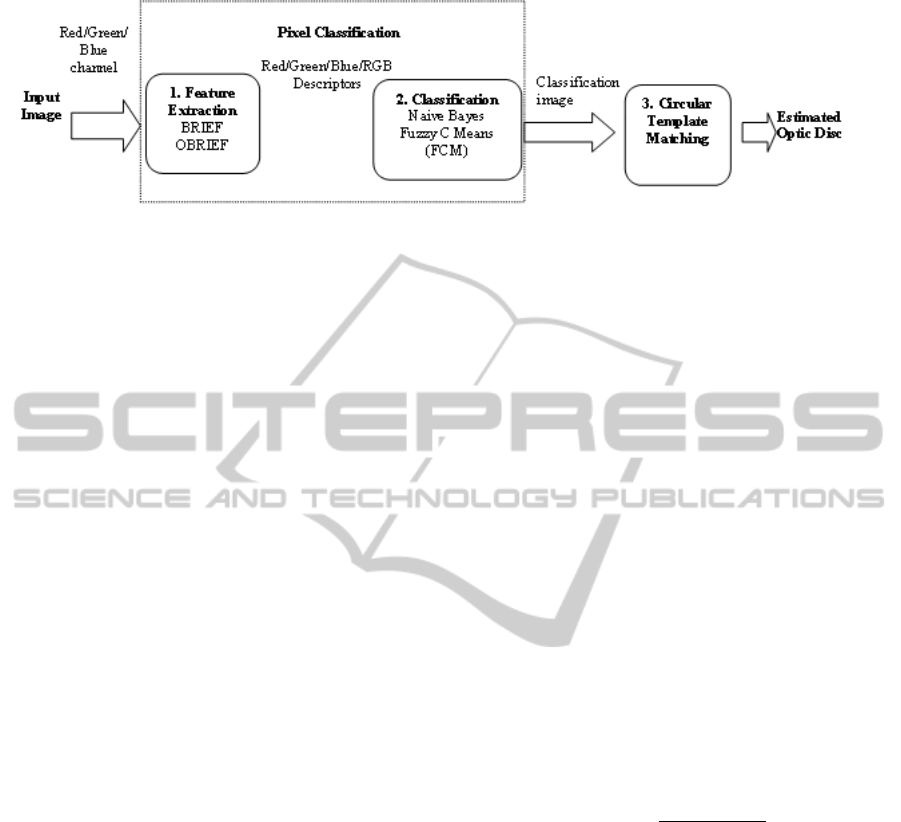
Figure 3: Flow Chart of the methods
methods used to classify/cluster each pixel into
one of two classes, ’optic disc’ and ’background’.
3. Circular Template Matching. This last stage is
to obtain the final circular approximation of the
optic disc. This will handle the gaps caused by
ingoing and outgoing blood vessels near the optic
disc boundary and will approximate the optic disc
boundary if not all of the boundary is detected.
3.1 Binary Robust Independent
Elementary Feature (BRIEF)
BRIEF (Calonder et al., 2010) uses binary vectors to
represent image patches. It takes a smoothed image
patch and computes the result of the binary test be-
tween sets of pairs of pixel intensities. The location
of the pixels pairs are predefined either randomly or in
systematic pattern and lies within the patch. The fea-
ture descriptor for a patch is then defined as a vector
of n binary tests.
Two important considerations when computing
BRIEF descriptors are the smoothing kernel to be
used and the spatial arrangement of the pixel pairs.
Smoothing is introduced to suppress noise, thus in-
creasing the stability and repeatability of the descrip-
tors (Calonder et al., 2012). However smoothing may
cause loss of spatial image detail,because of that we
adopted the method used in (Tar and Thacker, 2011),
i.e. we estimate the noise level beforehand and use
it as a threshold when calculating the BRIEF descrip-
tors. In this works, the test locations (the pixel pairs)
are defined randomly within the patch.
The formal definition of the BRIEF descriptor
used in our work is as follows:
A test τ defined on patch p of size SxS as
τ(p;x
¯
, y
¯
) =
1 if (p(x
¯
) - (p(y
¯
)) >Threshold
0 otherwise
(1)
where p(x
¯
) and p(y
¯
) are the pixel intensities at loca-
tions x
¯
and y
¯
.
The BRIEF descriptor is defined as the n bit vector
f
n
=
∑
1≤i≤n
2
i−1
τ(p;x
¯
i
, y
¯
i
) (2)
We choose S = 27 and n = 16. Other combinations
of S and n were considered and tested with a smaller
number of training cases. The above mentioned pa-
rameters were selected as they gave the best result.
The threshold is set to 3 times the estimated image’s
noise magnitude.
3.2 Naive Bayes Classifier
Naive bayes (Duda et al., 2001) is used as a sample of
supervised learning. It has the advantages of simplic-
ity, computational efficiency, and good classification
performance and in some cases is able to outperform
more sophisticated classifiers.
Since the BRIEF features are binary, given a finite
set of features then Bayes theorem can be expressed
as:
P(ω
i
|x) =
P(x|ω
i
)P(ω
i
)
P(x)
(3)
Where ω
i
is the i
th
class. P(ω
i
) is a priori probability
of class ω
i
, P(x|ω
i
) is the likelihood of feature vector
x given a class ω
i
and P(ω
i
|x) is the posterior prob-
ability of class ω
i
given observation x, i.e. the result
of the Bayes rule. P(x) is the normalisation constant.
We estimate P(ω
i
) and P(x|ω
i
) from the training data.
The decision rule used for classification is based on
maximum a posterior (MAP), i.e. choose the class
with the highest P(ω
i
|x).
We used Naives Bayes with two fold cross valida-
tion. BRIEF features from the optic disc and back-
ground are used to train the Naive Bayes.
3.3 Fuzzy C Means (FCM)
FCM clustering is selected as a sample of unsuper-
vised learning. One of the advantages of unsupervised
VISAPP2014-InternationalConferenceonComputerVisionTheoryandApplications
296

learning is that it is not dependent on the training data,
and thus it is generalisable to new cases. FCM is a
method of clustering where each point may belong to
one or more clusters with different degree of mem-
bership (Bezdek, 1981). The features with close sim-
ilarity in an image are grouped into the same clusters.
Similarity is defined as the distance from feature vec-
tors to the cluster’s centre.
FCM is based on minimisation of the objective
function in equation 4, by iteratively updating the
membership u
ik
and cluster centre v
i
:
J =
N
∑
k=1
C
∑
i=1
u
m
ik
kx
k
− v
i
k
2
(4)
where N is the number of data points, C is the number
of clusters, x
k
is the kth data point, v
i
is the ith cluster
centre, u
ik
is the degree of membership of kth in the
ith cluster and m is a constant greater than 1 (normally
2), used to determine the fuzziness of the clusters. In
this study the number of cluster is chosen as two, optic
disc and background cluster.
The membership degree, u
ik
and the cluster centre
v
i
are defined by:
u
ik
=
1
C
∑
j=1
(
kx
k
− v
i
k
kx
k
− v
j
k
)
2
m−1
(5)
v
i
=
N
∑
k=1
u
m
ik
x
k
N
∑
k=1
u
m
ik
(6)
Given the desired number of clusters and initial
value of cluster centres, the FCM will converge to a
solution for v
i
that represents a local minimum or sad-
dle point of the cost function J (Bezdek, 1981).
3.4 Circular Template Matching
To approximate the circular boundary of the optic disc
we use circular and elliptical template matching. The
templates are of various diameters and orientations
(see examples in Figure 4), and these templates will
be cross correlated with the classification result im-
ages. The matching process is done in parallel in the
four classification images from the red, green, blue
and RGB channel.
The correlation coefficient was used to present an
indication of the match between the template image
and the classification image. The final decision of the
good match is taken as the one with the highest corre-
lation value.
Figure 4: Samples of the template used.
4 TESTING AND RESULT
The image database used in this study is made up
of 196 images. 110 images are normal and 86 are
glaucomatous images. These images were kindly pro-
vided by Manchester Royal Eye Hospital.
The algorithm performance was evaluated by
measuring the overlap area, using an overlapping
score (O) between the ground truth optic disc region
and the approximated regions obtained from the de-
scribed approach, defined as below:
O =
Area(G ∩ S)
Area(G ∪ S)
(7)
where O is the overlap area, G is the ground truth re-
gion and S is the segmented region by the proposed
approach. An overlap area of ’1’ indicates perfect
agreement between ground truth and the proposed
approach. For the determination of CDR value, the
vertical length of the disc region is often measured.
Therefore average errors in the largest vertical length
of the disc region are also calculated.
The results are shown in Table 1 and Table 2. The
average overlap area between the ground truth and
the segmentation result by FCM and Naive Bayes are
0.85 and 0.84 for the normal set respectively. For the
glaucomatous set of images the overlapping score for
FCM and Naive Bayes is 0.77. In the classification
image result using FCM, the optic disc boundary is
more pronounced thus giving a slightly better perfor-
mance.
As expected the average overlapping area result in
the glaucomatous set is slightly lower than the normal
set. The reason is that glaucoma deforms the optic
disc shape making it less conforming to the standard
shape of our templates. In addition, a larger number
of images in this set show signs of atrophy. Atrophy
shares similar characteristic to the optic disc, thus at-
rophy regions are misclassified as optic disc pixels. In
the case of severe atrophy the image is either over seg-
mented or under segmented. Samples of segmented
optic discs are shown in Figure 5.
A good segmentation result is obtained in an im-
age with a good contrast and clear optic disc bound-
ary. The system also managed to get good approxima-
tion in an image with incomplete optic disc boundary
and the presence of mild atrophy. Poor segmentation
SegmentationofOpticDiscinRetinaImagesusingTexture
297
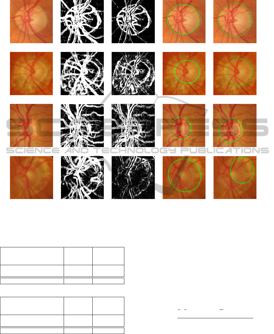
Figure 5: This figure illustrates the process of segmenting the optic disc, performed on the colour combination channel. The
first and fourth rows are images from the normal images set. The second and third row are images from the glaucomatous
set. From left to right: Original image, classification image using FCM, classification image using Naive Bayes, optic disc
boundary approximation using FCM and optic disc boundary approximation using Naive Bayes. The dotted line is the ground
truth and the green line is the approximated boundary.
Table 1: Disc segmentation result by the Fuzzy C Means.
Average
overlapping
ratio
Vertical
length
error (%)
Horizontal
length error
(%)
Normal 0.85 3.1 4.3
Glaucoma 0.77 5.8 6.0
All 0.81 4.5 5.2
Table 2: Disc segmentation result by the Naive Bayes.
Average
overlapping
ratio
Vertical
Length
error (%)
Horizontal
Length
Error (%)
Normal 0.84 4.9 5.2
Glaucoma 0.77 7.1 8.6
All 0.81 6 6.9
results are normally obtained from an image with ei-
ther severe atrophy (Figure 5:row 4), or with quite a
number of thick vessels passing in and out of the optic
disc (Figure 5:row 3) and those with irregular shape.
We also compared our result to another common
template matching approach that is the Hough trans-
form as implemented in (May, 2008). The Hough
Transform is performed based on the edges obtained
by the Canny edge detector. Vessel removal is imple-
mented prior to the edge detector. The evaluation used
in their work is based on calculating the discrepancy
(D) between two closed boundary curves or contour
described as:
D(G
c
, S
C
) =
1
2
{
1
n
n
∑
i=1
d(g
ci
, S) +
1
m
m
∑
i=1
d(s
ci
, G)}
G
d
(8)
G
c
and S
c
are the contours of the segmented area in
the ground truth and segmented images. d(a
i
, B) is
the minimum distance from point i on the contour A
to any point on the contour B. G
d
is the diameter of
the ground truth contour. A low discrepancy value
implies a better segmentation performance.
VISAPP2014-InternationalConferenceonComputerVisionTheoryandApplications
298

The comparison result is shown in Table 3. As can
be seen, our approach shows improvement in min-
imising the discrepancy over the Hough Transform
method. Figure 6 shows a sample image where the
optic disc is successfully segmented by all three meth-
ods (Row 1) and an image where our approach shows
a better segmentation result compared to the Hough
Transform (Row 2). In this particular case, the Hough
Transform is trapped by the strong optic cup bound-
ary.
Table 3: Average Discrepancy (D) by the three methods.
FCM Naive Bayes Hough Transform
Normal 0.06 0.06 0.10
Glaucoma 0.09 0.09 0.13
All 0.08 0.08 0.12
Figure 6: Comparisons of disc outlines determine by the
three method. From left to right: Optic disc boundary ap-
proximation based on clustering result by FCM clustering
and optic disc boundary approximation based on classifica-
tion result by Naive Bayes and optic disc approximation by
the Hough Transform. The dotted line is the ground truth
and the green line is the approximated boundary.
5 CONCLUSIONS AND FUTURE
WORKS
A method for optic disc segmentation is presented in
this paper. We demonstrate that the proposed method
is at least as reliable as other algorithms for the op-
tic disc segmentation with the advantages of com-
putational simplicity. An interesting property of our
method is the use of an illumination invariant texture
measurement to address the illumination issue of the
retina images. Furthermore, by making use of ma-
chine learning techniques in our approach, we can ex-
ploit the knowledge of the characteristics of the optic
disc in the segmentation process.
Nonetheless, the method has several limitations
which we aim to address in future research. We used
training data to model the optic disc characteristic
with the hope of better discrimination between optic
disc and background pixels (including vessels and at-
rophy pixels). However, some miss classification be-
tween pixels on the vessel boundaries, atrophy and
optic disc boundary do occur in some of the images.
Thus in future we intend to (1) implement a rotation
invariant version of BRIEF as an attempt to reduce
miss classification of vessels and (2) ensure that data
used for training the Naive Bayes includes sufficient
number of atrophy pixels so that the result may im-
prove. At the moment the pixels used in the training
data were randomly selected.
Another problem is the use of circular/elliptical
template matching. Quite often, this approach fails to
get good segmentation in cases where the optic disc
is not of ’standard’ shape. Therefore we are currently
looking at ways to trace the boundary from the classi-
fication image guided by the obtained circumference
given by the template matching approach.
REFERENCES
Bezdek, J. C. (1981). Pattern recognition with fuzzy objec-
tive function algorithms. Kluwer Academic Publish-
ers.
Calonder, M., Lepetit, V., Ozuysal, M., Trzcinski, T.,
Strecha, C., and Fua, P. (2012). Brief: Computing
a local binary descriptor very fast. Pattern Analy-
sis and Machine Intelligence, IEEE Transactions on,
34(7):1281–1298.
Calonder, M., Lepetit, V., Strecha, C., and Fua, P. (2010).
Brief: binary robust independent elementary features.
In Computer Vision–ECCV 2010, pages 778–792.
Springer.
Congdon, N. G., Friedman, D. S., and Lietman, T. (2003).
Important causes of visual impairment in the world
today. JAMA: the journal of the American Medical
Association, 290(15):2057–2060.
Cree, M. J., Olson, J. A., McHardy, K. C., Sharp, P. F.,
and Forrester, J. V. (1999). The preprocessing of
retinal images for the detection of fluorescein leak-
age. Physics in Medicine and Biology, 44(1):293–308.
Cited By (since 1996):18.
Duda, R., Hart, P., and Stork, D. (2001). Pattern classifica-
tion. Wiley, pub-WILEY:adr, second edition.
Foracchia, M., Grisan, E., and Ruggeri, A. (2004). Detec-
tion of optic disc in retinal images by means of a geo-
metrical model of vessel structure. IEEE Transactions
on Medical Imaging, 23(10):1189–1195.
Foracchia, M., Grisan, E., and Ruggeri, A. (2005). Lu-
minosity and contrast normalization in retinal images.
Medical Image Analysis, 9(3):179–190.
Grisan, E., Giani, A., Ceseracciu, E., and Ruggeri, A.
(2006). Model-based illumination correction in reti-
nal images. In Biomedical Imaging: Nano to Macro,
2006. 3rd IEEE International Symposium on, pages
984–987. IEEE.
SegmentationofOpticDiscinRetinaImagesusingTexture
299

Hoover, A. and Goldbaum, M. (2003). Locating the optic
nerve in a retinal image using the fuzzy convergence
of the blood vessels. Medical Imaging, IEEE Trans-
actions on, 22(8):951–958.
Joshi, G. D. and Sivaswamy, J. (2008). Colour retinal image
enhancement based on domain knowledge. In Com-
puter Vision, Graphics & Image Processing, 2008.
ICVGIP’08. Sixth Indian Conference on, pages 591–
598. IEEE.
Joshi, G. D., Sivaswamy, J., and Krishnadas, S. (2011). Op-
tic disk and cup segmentation from monocular color
retinal images for glaucoma assessment. Medical
Imaging, IEEE Transactions on, 30(6):1192–1205.
Kass, M., Witkin, A., and Terzopoulos, D. (1988). Snakes:
Active contour models. International journal of com-
puter vision, 1(4):321–331.
Lowell, J., Hunter, A., Steel, D., Basu, A., Ryder, R.,
Fletcher, E., and Kennedy, L. (2004). Optic nerve
head segmentation. Medical Imaging, IEEE Trans-
actions on, 23(2):256–264.
May, M. (2008). Automatic Detection of the Optic Disc
Within Retinal Images. Master’s thesis, University of
Manchester, UK.
Morris, D. and Donnison, C. (1999). Identifying the neu-
roretinal rim boundary using dynamic contours. Im-
age and Vision Computing, 17(3):169–174.
Muramatsu, C., Nakagawa, T., Sawada, A., Hatanaka, Y.,
Hara, T., Yamamoto, T., and Fujita, H. (2011). Au-
tomated segmentation of optic disc region on retinal
fundus photographs: Comparison of contour model-
ing and pixel classification methods. Computer meth-
ods and programs in biomedicine, 101(1):23–32.
Ricci, E. and Perfetti, R. (2007). Retinal blood vessel
segmentation using line operators and support vector
classification. Medical Imaging, IEEE Transactions
on, 26(10):1357–1365.
Spencer, T., Olson, J., McHardy, K., Sharp, P., and For-
rester, J. (1996). An image-processing strategy for the
segmentation and quantification of microaneurysms in
fluorescein angiograms of the ocular fundus. Comput-
ers and Biomedical Research, 29(4):284–302.
Tar, P. and Thacker, N. (2011). A quantitative representation
for segmentation of martian images. Technical report,
ISBE, Medical School, University of Manchester.
Walter, T. and Klein, J.-C. (2002). A computational ap-
proach to diagnosis of diabetic retinopathy. In Pro-
ceedings of the 6th Conference on Systemics, Cyber-
netics and Informatics (SCI2002), pages 521–526.
Wang, Y., Tan, W., and Lee, S. C. (2001). Illumination nor-
malization of retinal images using sampling and inter-
polation. In Medical Imaging 2001, pages 500–507.
International Society for Optics and Photonics.
Winder, R., Morrow, P., McRitchie, I., Bailie, J., and Hart,
P. (2009). Algorithms for digital image processing in
diabetic retinopathy. Computerized Medical Imaging
and Graphics, 33(8):608 – 622.
Youssif, A. A., Ghalwash, A. Z., and Ghoneim, A. S.
(2007). A comparative evaluation of preprocessing
methods for automatic detection of retinal anatomy. In
Proceedings of the Fifth International Conference on
Informatics and Systems (INFOS 07), pages 24–30.
VISAPP2014-InternationalConferenceonComputerVisionTheoryandApplications
300
