An Inverse Distance-based Potential Field Function for Overlapping
Point Set Visualization
Jevg
¯
enijs Vihrovs, Kri
ˇ
sj
¯
anis Pr
¯
usis, K
¯
arlis Freivalds, P
¯
eteris Ru
ˇ
cevskis and Valdis Krebs
Institute of Mathematics and Computer Science, University of Latvia, Rain¸a bulv
¯
aris 29, LV-1459, Riga, Latvia
Keywords:
Information Visualization, Implicit Surfaces.
Abstract:
In this paper we address the problem of visualizing overlapping sets of points with a fixed positioning in a
comprehensible way. A standard visualization technique is to enclose the point sets in isocontours generated
by bounding a potential field function. The most commonly used functions are various approximations of
the Gaussian distribution. Such an approach produces smooth and appealing shapes, however it may produce
an incorrect point nesting in generated regions, e.g. some point is contained inside a foreign set region. We
introduce a different potential field function that keeps the desired properties of Gaussian distribution, and
in addition guarantees that every point belongs to all its sets’ regions and no others, and that regions of two
sets with no common points have no overlaps. The presented function works well if the sets intersect each
other, a situation that often arises in social network graphs, producing regions that reveal the structure of their
clustering.
1 INTRODUCTION
Point sets emerge from the study of many real-world
data structures, from social networks to geographical
maps. The sets identify important groups of objects
inside the structure, for instance, scientific article co-
authorship (Santamara and Thern, 2008) or social cir-
cles in organizations (Krebs, 2007). Overlaps often
occur naturally in such graphs, with sets sharing com-
mon intermediary vertices. For example, human and
biological networks rarely cluster in clean ways, and
one vertex may belong to many groups.
After the identification of different point sets in
the given data, there is still the problem of presenting
this information in a quickly and easily comprehensi-
ble way. In order for the visualization of overlapping
point sets to be effective, it should adhere to various
criteria. Firstly, it should be unambiguous: the user
should be able to identify the sets and their points,
as well as their overlaps, without any misunderstand-
ings. It should also represent the geometrical layout
of the points themselves as closely as possible. In this
paper we deal with visualizing point sets that have an
arbitrary, but fixed positioning.
The common approach in visualization is to en-
close the points of each set in a region that represents
this set, forming an Euler diagram. There are several
works that list the desirable properties of visualiza-
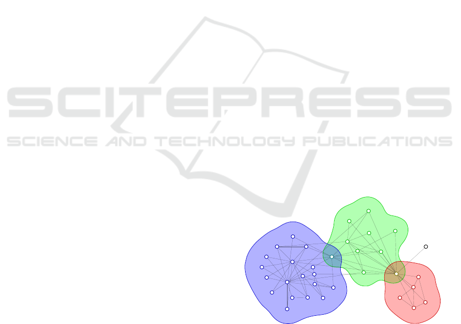
Figure 1: An example of the proposed visualization. There
are three overlapping point sets, which correspond to vertex
clusters in the given graph. In this example edges do not
affect the visualization.
tions that produce such regions (Rosenthal and Lin-
sen, 2009; Dinkla et al., 2012). Here we present a
brief summary.
P1 Each point of a set is contained inside the region
of this set.
P2 Each point not present in a set is not contained
inside the region of this set.
P3 The regions of two different sets must have over-
laps only where there is a point that belongs to
both of the sets.
P4 The regions must have a strict boundary that sep-
29
Vihrovs J., Pr¯usis K., Freivalds K., Ru
ˇ
cevskis P. and Krebs V..
An Inverse Distance-based Potential Field Function for Overlapping Point Set Visualization.
DOI: 10.5220/0004681100290038
In Proceedings of the 5th International Conference on Information Visualization Theory and Applications (IVAPP-2014), pages 29-38
ISBN: 978-989-758-005-5
Copyright
c
2014 SCITEPRESS (Science and Technology Publications, Lda.)

arates the included and excluded space.
P5 The boundary of the region should stay close to
the points of the set.
P6 The boundaries of the regions should be suffi-
ciently smooth.
P7 The region of one set should be connected.
A widely used visualization method is to compute
the regions by bounding a potential field function.
The advantages are the smooth shape borders and the
flexibility of the result, as the function parameters can
be adjusted to obtain a better visualization. The main
problems are ensuring the correct membership of the
points (P1, P2) and region overlapping (P3), as well
as maintaining each region connected (P7). Tradition-
ally, most potential functions are based on the Gaus-
sian distribution function (Blinn, 1982; Gross et al.,
1997; Sprenger et al., 2000) or quadratic polinomial
functions (Watanabe et al., 2007; Collins et al., 2009).
These functions naturally satisfy properties P4-P6.
The main problem with such functions is main-
taining the membership properties P1-P3. If each set
region is calculated ignoring the influence of the for-
eign points, then P1 holds, but P2 and P3 are com-
pletely ignored. To mitigate this, the foreign points
are assigned a negative potential, thus repelling the
influence of the points of the given set. This im-
proves P2 and P3 (though does not fully satisfy ei-
ther), but violates P1, as negative potentials can over-
whelm positives ones even directly at a point. To limit
the effect this has on P1, smaller weights are often
used for negative potentials. However, this weak-
ens the improvements to P2 and P3. In particular,
only when negative and positive potentials are equal
does the following hold: if two sets share no common
point, their regions do not overlap, which is important
in cases with no overlapping sets.
In this work we address this problem and propose
a different potential field function that always pro-
duces visualization with correct point membership,
and visually still behaves much like the mentioned
potential functions. It is very similar to Gaussian-
based methods in isocontour appearance and satisfies
the same properties P4-P6. In addition, when using
our function with equal negative and positive weights
as described earlier, it is guaranteed to satisfy proper-
ties P1, P2 concerning the membership of the points.
Thus it also guarantees the property P3 for every two
sets with no common points. We show the results of
the visualization on different artificial and real-world
examples and compare them to other potential func-
tions. The function has also two parameters that allow
to adjust the size and appearance of the produced re-
gions.
Maintaining property P7 is a topological problem,
and cannot be solved by a specific potential func-
tion design. Still, it can be ensured using standalone
techniques such as including the edges of each set’s
spanning tree when computing the potential function
(Collins et al., 2009), but usually at the cost of ignor-
ing correct overlap properties P2 and P3. We show
how this method works with the proposed function.
However, as the proposed function is designed to im-
prove properties P1-P3, this leads to unusual visual
behavior. Without this property the region of each
set can consist of multiple disconnected shapes. In
our examples, we use color-coding to differentiate be-
tween set regions.
2 RELATED WORK
There have been a substantial number of works that
deal with overlapping point set visualization. The
problem is highly relevant in visualizing graph vertex
clusters in graph drawing, and many approaches are
described in the context of graph clusters (Gansner
et al., 2010; Balzer and Deussen, 2007; Van Ham and
Van Wijk, 2004; Heer and Boyd, 2003).
The main tasks pursued in most visualizations are
maintaining connectivity of the regions of a set (P7)
and point region membership (P1-P3). The connectiv-
ity is very important in the sense that it allows the user
to quickly identify a particular set. The correctness
of the sets’ overlaps may be crucial in understanding
the membership of the points and the relationships
of the sets. Both these properties may be conflict-
ing: if the positioning of the points is fixed, it is fre-
quently not possible to ensure connectivity and elimi-
nate all unnecessary region overlaps. It is also impor-
tant whether the layout of the points can be changed
or not; various algorithms of point positioning may
greatly improve the readability of the visualization.
The most straightforward approach for obtaining
the region of a set is to obtain its convex hull, used,
for example, in (Heer and Boyd, 2003; Santamara and
Thern, 2008). Here, the boundaries of the convex
hulls are smoothed by using B
´
ezier curves. However,
the convex hull approach ignores the P2 and P3 prop-
erties, and many points may happen to reside inside
foreign set regions. This is addressed in (Byelas and
Telea, 2009), which describes visualization of UML
diagrams. The areas where foreign elements overlap
the convex hull are excluded from the region heuristi-
cally, and afterwards the resulting polygon is shrunk
inwards to better represent the layout of the elements
in the set. The borders of the regions are also softened
which achieves a more natural look of the shapes.
IVAPP2014-InternationalConferenceonInformationVisualizationTheoryandApplications
30

A more sophisticated method that also computes
discrete hulls is proposed in (Simonetto et al., 2009).
The intersection graph of the sets (which is planar) is
built and positioned using a force-directed algorithm
(Di Battista et al., 1998). Then a polygonal skeleton is
built around the graph vertices, and the points are in-
serted inside the corresponding polygons; these poly-
gons are then expanded by applying the force-directed
layout algorithm several more times. The resulting
visualization has correct point membership, and each
set region is connected, thus all the constraints P1-P3,
and P7 are fully satisfied. Still, this visualization can
be applied only when the positioning of the points is
not important.
Another method is to use the Voronoi diagram of
the given points to create the space partitioning for
the visualization. A simple application of such ap-
proach for visualizing self-organizing maps can be
found in (Matsumoto et al., 2008). The result fully
ensures all the membership constraints P1-P3, and is
very simple to implement. However, the regions have
many sharp edges and all borders are shared (P6 does
not hold). Another problem is the long and sharp re-
gion parts that do not contain any set vertices, which
are common in Voronoi diagrams, as these parts dis-
tort the regions and lessen readability, violating P5.
GMap (Gansner et al., 2010) mitigates this by insert-
ing many artificial points in the diagram around the ar-
eas of interest. A particular technique for smoothing
the boundaries of the regions is described in (Rosen-
thal and Linsen, 2009), which also uses Voronoi dia-
grams. They create the region boundaries by using the
Voronoi diagram to obtain a hull of the set and then
drawing a distance field around this hull. This does
not, however, work on boundaries between adjacent
or intersecting regions. A problem with all Voronoi-
based methods is that they do not ensure region con-
nectivity.
The approach used in this work is to compute the
regions for point sets by using a potential field func-
tion. The value of influence of a point in the given
space is defined by the potential function, and the to-
tal influence of a point set in some location is the sum
of influences for all the points in the set. Then the
region for a set is obtained by thresholding the total
influence of this set.
The properties of such visualization depend on the
choice of the potential field function. Most standard
potential functions are based on the Gaussian distribu-
tion. Its main advantage is the contour smoothness of
the regions, they look similar to hand-drawn. One of
the first analyses of such a potential function appears
in (Blinn, 1982). It also describes how the “blobbi-
ness” of the visualization can be adjusted using the
parameters of the function.
Another type of potential functions are polyno-
mial approximations of Gaussians that are faster to
compute and produce nearly identical results, e.g.
(Balzer and Deussen, 2007). Also used are bounded
quadratic functions (Watanabe et al., 2007; Collins
et al., 2009), they generate similar results.
This approach has been widely applied in point set
visualization. Some works visualize and cluster point
sets in 3D (Sprenger et al., 2000; Balzer and Deussen,
2007). The latter also focuses on hierarchical depic-
tion of a clustered graph. To avoid incorrect overlaps
of different set regions, one can assign negative poten-
tial to point of foreign sets, which is noted in (Blinn,
1982), and used in (Gross et al., 1997; Watanabe et al.,
2007; Collins et al., 2009).
Bubble Sets (Collins et al., 2009) directly focus
on 2D point set visualization; while it also uses a po-
tential field function and negative influences for for-
eign set points, it maintains P7 by using the edges of
a spanning tree of each set in addition to the vertices
when computing the potential functions. However,
these edges from different sets can overlap, violating
P3.
Other novel methods include Euler diagrams with
connected regions (Riche and Dwyer, 2010), as well
as Kelp diagrams (Dinkla et al., 2012), which focus
primarily on region connectivity in visualizing points
with fixed geometrical layout.
3 THE POTENTIAL FUNCTION
We are given a set of points and the subsets we have to
visualize, along with a geometrical positioning of the
points in an Euclidean space. For clarity, we will call
the given points the vertices (from the use cases of
representing social graphs), to avoid confusion with
spatial points. For each set, we independently com-
pute a function which assigns a real number to each
point denoting the set’s influence on it. Vertices be-
longing to the set positively influence the value of
the function, whereas other vertices influence it neg-
atively. The amount a vertex influences a point is de-
termined by their distance.
After calculating the function for a set, the shape
for this set is extracted using a fixed threshold. We de-
scribe the potential function in Sect. 3.1. In Sect. 3.3,
we discuss the specifics of the implementation.
3.1 Function Description
Suppose we are given N non-empty sets S
1
...S
N
where ∀i : S
i
⊆ V , and V is the set of all the vertices.
AnInverseDistance-basedPotentialFieldFunctionforOverlappingPointSetVisualization
31

Some vertices can also belong to no set. These ver-
tices in any case negatively influence the value of the
function for all sets.
For the visualization, we need the vertices to be
geometrically positioned. The positioning can be ex-
pressed by a function P : V → R
n
that assigns a po-
sition to each vertex in a n-dimensional Euclidean
space. Clearly, in practice, the visualization can be
meaningful to users when n ≤ 3. For use case with-
out a predefined layout, constructing the function P
is itself a separate, well-studied problem(Di Battista
et al., 1998). In this work, we do not propose any
new positioning methods, and the visualization itself
does not require any special positioning. For clus-
tered graphs, we will often use a positioning based on
a force-directed layout algorithm.
The field function approach works as follows:
first, define the influence of a vertex v with respect
to a point p, which is a function I(v, p). Then the in-
fluence of a vertex set S on a point p is defined as the
sum of the influence of its vertices:
I(S, p) =
∑
v∈S
I(v, p). (1)
The potential field function for set S
i
at a point p is
defined as the difference between the influence of this
set and the total influence of all other vertices:
F
i
(p) = I(S
i
, p) − w · I(V \ S
i
, p) (2)
All the vertices that belong to the i-th set influence
the value of the function positively, whilst all other
vertices influence it negatively. The nonnegative pa-
rameter w is the weight of negative influence, which
is usually less than 1 (i.e. the weight of the positive
influence).
To obtain a shape that represents the i-th set, use a
nonnegative threshold t. The region of the vertex set
is defined to be the set of points such that for any point
p in the set the inequality F
i
(p) > t holds. By adjust-
ing the value of t the shapes can be made smaller or
larger. In practice, it can be difficult to estimate the
shape size from t, therefore we adjust the desired ra-
dius of the shape of a single vertex R
t
and set t to be
the influence of a single vertex at distance R
t
.
Since the influence of the vertices belonging to S
i
is taken with a positive sign and the influence of other
vertices with a negative sign, vertices not belonging
to the set repel its shape.
As the function I(v, p) we use the following:
I(v, p) = max(kP(v) − pk
−b
− m,0) (3)
where b and m are nonnegative constants (parame-
ters). We also use the weight w = 1 (we show later this
contributes to an important property of the function).
When kP(v) − pk = 0, influence I(v, p) is defined as
lim
x→0
1
x
= +∞.
There can also be a situation when two or more
vertices have equal positions, where by (3) it is not
clear what value should F
i
take. For example, there
can be one vertex v
1
from set i and two other v
2
, v
3
from set j in the same point p. For all three vertices
the influence in this point is equal to infinity, so F
i
formally is undefined. In this case F
i
should be equal
to −∞, since for all other points q the value of F
i
is
−I(v
3
,q) = I(v
1
,q) − I(v
2
,q) − I(v
3
,q). So in such
situations, if the number of set i vertices in point p
is less than the number of foreign set vertices in this
point, then F
i
(p) should be equal to −∞, and +∞ or 0
if it is greater or equal respectively. This may not be
very important as it affects only individual points but
should be noted during implementation.
Parameter b regulates the slope of the function.
When b grows larger, the function decreases much
faster when distance is greater than 1. Visually this
adjusts how strongly the blobs of the vertices interact
with each other. Fig. 2 shows the graphs of the func-
tion with different b values (m = 0). The threshold
b was chosen so that for each function the radius of
a single blob would be constant. When m is small,
the blobs of nearby vertices meld together. When b is
large, they appear as overlapping circles.
I
distance
b = 0.2
b = 1
b = 2
b = 20
(a) (b)
(c) (d)
Figure 2: Graphs of the influence function with different b
values. This example shows how b affects blob interaction:
(a) b = 0.2; (b) b = 1; (c) b = 2; (d) b = 20. The radius of
a single blob R
t
is the same in all examples.
The value m is subtracted to set function values
IVAPP2014-InternationalConferenceonInformationVisualizationTheoryandApplications
32

to 0 starting from a certain distance. The purpose of
this is to limit the maximum effect radius of a sin-
gle vertex, preventing large concentrations of vertices
from accumulating a large radius of the correspond-
ing region with respect to other regions that contain
less vertices. This is shown in Fig. 3: m normalizes
the radiuses of the small and large set regions. Again,
as with threshold, we regulate m with the use of the
value R
m
, which is defined as the distance at which
the value of influence of a single vertex is equal to 0.
It is clear that R
m
should be greater than R
t
; we mostly
set the value of R
m
to be a multiple of R
t
.
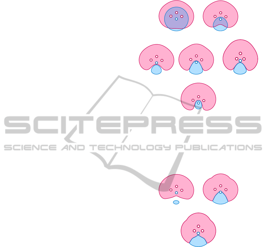
(a) (b)
Figure 3: The effect of parameter m on the consistency of
region radiuses: (a) R
m
is unbounded (m = 0), the larger set
region has a much larger radius then the smaller set region;
(b) R
m
= 2.5R
t
, the radiuses of the regions are almost the
same.
3.2 Properties and Comparison
In this section we discuss how the presented func-
tion deals with properties P1-P3 and how it com-
pares to already known functions. As influence func-
tion I(v, p) we also consider the Gaussian distribu-
tion function e
−
x
2
2σ
2
and quadratic polynomial func-
tion (max(r − x,0))
2
, where x = kP(v) − pk. For
Gaussian distribution function, standard deviation pa-
rameter σ also adjusts blobbiness. Overall the pro-
posed function keeps the desired properties of these
functions, and in addition guarantees correct point re-
gion membership because the potential function di-
verges to plus infinity at x = 0.
A simple example in Fig. 4 shows that the pro-
posed function maintains the visual appearance of
Gaussian distribution and quadratic polynomial po-
tential functions. Of course, each function has its pa-
rameters that adjust the blobbiness and size of the re-
gions, so each can be used to produce different visu-
alizations with the same example case. However, the
figure shows that all three functions can be adjusted
to produce similar-looking results.
Further we examine how these functions satisfy
(a) (b)
(c)
Figure 4: A simple example of how the proposed function
maintains the appearance of common potential functions:
(a) Gaussian distribution; (b) quadratic polynomial; (c) pro-
posed function.
the membership properties P1-P3. In contrast to other
functions, the proposed function guarantees proper-
ties P1, P2. It also ensures property P3 for sets with
no common points.
The property P1 is easy to establish for any po-
tential function by taking w = 0 in (2), i.e. ignoring
foreign vertex influence for the current set. This intro-
duces many unwanted region intersections, thus prop-
erties P2 and P3 are not maintained. This is shown
in Fig. 5 (a) with Gaussian distribution (of course
it happens with any potential function): the blue and
red regions almost completely overlap (they should
not since the two sets do not have any vertex in com-
mon), besides the blue region swallows all vertices of
the red region.
This means that if we want to remove unnecessary
region overlaps or ensure correct vertex membership,
we have to adjust the value of w. Fig. 5 (b) shows
the same example with Gaussian distribution and w =
0.5. The vertex membership is correct, but the regions
still overlap. Fig. 5 (c) uses Gaussian with w = 1,
i.e. the negative potential has the same weight as the
positive. In this case the two regions do not overlap,
but the red region swallows the single blue vertex.
That is, in fact, an important property when w = 1,
which holds for any potential function. If two sets
have no vertices in common, then their regions do not
overlap (this is actually a special case of the P3 prop-
erty). The proof is trivial: suppose the total positive
influences of the two sets at some spatial point are I
1
and I
2
. Only one of the values I
1
− I
2
and I
2
− I
1
can
be positive, thus only one can be greater than thresh-
old t. Other set vertices do not change this property,
since for each spatial point the influence from them is
subtracted from both of the given set total influences.
This property is very important if we need to visu-
alize sets with no intersections: then no two regions
will have any overlaps. Therefore we would want to
keep it while also ensuring correct vertex member-
AnInverseDistance-basedPotentialFieldFunctionforOverlappingPointSetVisualization
33
ship. We examine this property for a small example
with a fixed R
t
.
Using a Gaussian function with a fixed parameter
σ, as it is shown in Fig. 5 (a)-(c), all of the mentioned
properties at once are not achievable. In the given ex-
ample, we can change σ (from 2.5 to 3.5), and obtain
a correct visualization, see Fig. 5 (d); however, this
is an unstable improvement and slightly adjusted ver-
tex positions again produce an incorrect visualization
even with the new σ, see Fig. 5 (e). In addition, σ also
regulates blobbiness and it is not desirable to adjust it
in order to maintain correctness.
With the proposed function all of the above is
guaranteed in the visualization, see Fig. 5 (f). Firstly,
we keep weight w = 1, so non-intersecting sets will
have no overlaps between their regions. Secondly,
the potential function is based on inverse distance and
reaches positive infinity at distance 0, regardless of
the function parameters. Thus properties P1 and P2
are ensured: each vertex will always be inside the re-
gions of the sets it belongs to and will not be inside
the regions of the sets it doesn’t belong to. This al-
lows using the parameters b and m to adjust the visual
quality of the result, while the membership of the ver-
tices will always be correct.
The only case when P1 and P2 do not hold is in
the same case if several different set vertices are in the
same position p. However, it is obviously impossible
to satisfy these properties with any visualization in
this case.
Using a quadratic polynomial function produces
results similar to those of using a Gaussian function,
see Fig. 6. Parameter r can be adjusted to regulate the
blobbiness. The red region swallows the blue vertex
in Fig. 6 (a), when r = 1.4R
t
. Again, it can be solved
by adjusting r to 1.02R
t
(see Fig. 6 (b)), and again
this solution is unstable and doesn’t work when the
vertex positions are changed slightly (see Fig. 6 (c)).
The example uses the same R
t
in all cases, but
a vertex positioning producing similar results can be
obtained for any R
t
. In practice, changing the radius
of the blobs is also unwanted if we need to obtain
shapes of particular size. With the proposed function
there is no need for fine-tuning to obtain a correct ver-
tex membership visualization.
It should be noted that the situation with P3 is dif-
ferent if two sets do have some vertices in common.
As it was shown that any vertex belonging to a set will
reside inside the region of this set, a vertex belonging
to two sets will also always reside in some intersec-
tion of their regions. However, among all overlaps of
the regions, there can be some that contain no vertices
from any of the given sets. These overlaps may be un-
wanted since they do not hold any semantic meaning
(a) (b)
(c) (d) (e)
(f)
Figure 5: Comparison with the Gaussian distribution func-
tion. The example shows two non-intersecting sets: 1 vertex
(blue); 3 vertices (red). In this example the threshold radius
R
t
is the same for all six cases. (a) Gaussian, σ =
R
t
/2.5,
w = 0. (b) Gaussian, σ =
R
t
/2.5, w = 0.5. (c) Gaussian,
σ =
R
t
/2.5, w = 1. (d) Gaussian, σ =
R
t
/3.5, w = 1. (e) Dif-
ferent vertex positioning, Gaussian, σ =
R
t
/3.5, w = 1. (f)
The proposed function, b = 2, R
m
= 2R
t
.
(a) (b)
(c)
Figure 6: Quadratic polynomial function (max(r − x, 0))
2
results with the same example and the same R
t
: (a) r =
1.4R
t
; (b) r = 1.02R
t
; (c) Different vertex positioning, r =
1.02R
t
.
of set relationship, see Fig. 7 (a). Still, such over-
laps can also contribute to the smooth region borders,
see Fig. 7 (b); without them, the image would not
look natural. Generally, this problem has a topologi-
cal nature and most probably cannot be solved solely
through potential function design.
3.3 Implementation
In this section we discuss the implementation
specifics of the proposed potential function. We use a
radial sweep algorithm to find the region boundaries
IVAPP2014-InternationalConferenceonInformationVisualizationTheoryandApplications
34

(a) (b)
Figure 7: Unnecessary region overlaps (with the proposed
potential function): (a) the highlighted overlap is unwanted;
(b) the highlighted overlaps are not necessary, but manda-
tory for smooth shape borders. Vertices that have black bor-
ders in each example belong to all sets.
for each set (marching squares could be used as well),
which are simplified using the Douglas-Peucker algo-
rithm (Douglas and Peucker, 1973). For high-quality
images (as in this paper) we also interpolate these
polygons with splines (Hobby, 1986).
One aspect of the implementation of our poten-
tial function is the possibility of infinity values. In
fact, due to datatype restrictions (for example, float-
ing point) such values could be achievable not only
exactly at a vertex, but also within some ε-distance
from the vertex. This problem can be solved by ad-
justing the used datatype for our function specifics:
• if the operation would cause the value of a vari-
able to overflow, it should take the special ∞-value
with an appropriate sign (the floating point stan-
dard guarantees this);
• if an ∞-value is added a value which is not an ∞-
value with the opposite sign, the result should re-
main the same ∞-value (the floating point stan-
dard guarantees this);
• if an ∞-value is added to an ∞-value with the op-
posite sign, the result should be 0 (this is different
from the floating point standard).
Still, in our implementation we used the standard
floating point datatype, as it is fully sufficient in prac-
tice and produces no visible errors, because such ε-
regions are negligible in size.
Another aspect of the implementation is choosing
appropriate values for b, m and t. Recall the following
auxiliary parameters we used in the previous section:
R
t
— the desired radius of the shape of a single ver-
tex; R
m
— the distance where the influence of a sin-
gle vertex reaches 0. These parameters can be used in
the implementation to adjust the look of the visualiza-
tion. We advise to set R
m
to be some multiple of R
t
,
for example, R
m
= 2R
t
. We use the following rules to
compute the actual parameters for the function:
• b = 2, but adjust in real-time if needed.
• m = R
−b
m
.
• t = R
−b
t
− m, provided R
m
> R
t
.
The running time of the implementation is mainly
dependent on the particulars of the radial sweep or
marching squares algorithm used. The only time-
consuming part connected with the function is the
calculation of the influence on the given scalar field,
which is essentially O((set count) · (vertex count) ·
(field size)). There are a few worthy optimizations
to this:
• since F
i
(p) = I(S
i
, p) − I(V \ S
i
, p), first calculate
only I(S
i
, p): if it is less than the used threshold t,
there is no need to calculate I(V \ S
i
, p);
• if the distance kP(v)− pk is greater than R
m
, then
the influence is 0 and there is no need to take v
into account for point p;
• to avoid expensive exponentiation in kP(v) −
pk
−b
, the value of b = 2 can be used, leaving only
the inverse of the easily computable squared dis-
tance between v and p.
4 CASE STUDIES
In this section we demonstrate our visualization on
several real-world examples and compare it to the
Gaussian distribution-based visualization. We show
that in cases where the Gaussian distribution works
well, so does the proposed function. In addition, we
show that our function can be used to achieve a good
result where that is not possible using the Gaussian
distribution. We focus on the Gaussian distribution
function, as quadratic polynomial potential functions
produce essentially the same results.
The first example shows that the proposed func-
tion can be used to obtain similar results to those of
the Gaussian distribution function, see Fig. 8. The lat-
ter works well in this example, and we have produced
essentially the same result using our function. The
example itself demonstrates a small company with
four work locations. The central red cluster corre-
sponds to the company headquarters. Each vertex
in the graph represents an employee, colored accord-
ing to the location they work at. Graph edges de-
note frequent, work-related communications between
employees. Cluster overlaps reveal which employees
frequently interact with other locations. Besides the
comparison of the functions, this example shows how
this visualization can be used to depict graph overlap-
ping clustering (Krebs, 2007).
AnInverseDistance-basedPotentialFieldFunctionforOverlappingPointSetVisualization
35
(a) (b)
Figure 8: This figure illustrates a visualization of a simple real-world overlapping set example: (a) Gaussian distribution; (b)
the proposed function. There are no difficulties in ensuring correct point membership for both functions in this case. The
example shows that our function is able to produce results that are very similar to the visualization with Gaussian distribution
function. Both cases illustrate that this visualization method works well with graph clustering.
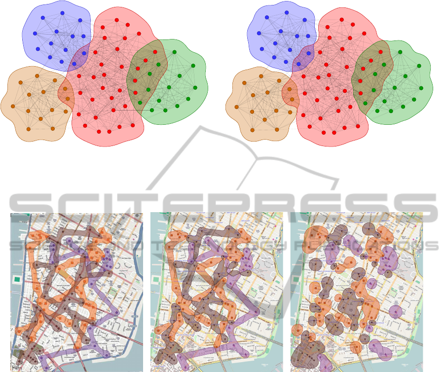
(a) (b) (c)
Figure 9: Hotels (orange), subway stations (brown), and medical clinics (purple) in Manhattan: (a) Bubble Sets (Collins et al.,
2009); (b) our function with spanning tree edges added to the visualization; (c) our function without any modifications. This
example shows how region connectivity can be ensured while using our function.
In the second example we compare our visual-
ization with Bubble Sets (Collins et al., 2009), see
Fig. 9 and illustrate how their method of ensuring re-
gion connectivity works with the proposed method.
The example depicts the locations of hotels, subway
stations and clinics in Manhattan. Case (a) shows
the Bubble Sets result. It uses a quadratic polyno-
mial function as the potential field function, and en-
sures region connectivity by assigning potential to the
edges of a (not necessary the minimum) spanning tree
of the set vertices in addition to the vertices them-
selves. When computing the influence of an edge on
a point the standard point-segment distance is used.
As a result the regions have unwanted overlaps, many
of which, however, contribute to region connectivity.
In case (b) we have applied the same spanning tree
method with our function. In addition to maintain-
ing connectivity, in our visualization there are also no
region overlaps. The function properties lead to in-
teresting behavior at edge intersection points, where
each of the regions is connected by a single point. We
leave it to the reader to decide whether such a result
is aesthetically pleasing. In case (c) we apply our vi-
sualization without any modifications.
In the last example we visualize a part of the hu-
man disease network described in (Goh et al., 2007),
see Fig. 10. In this graph, diseases are linked by
common genetic associations, with the sets denoting
various types of disease. This graph contains no set
overlaps, so using equal weights for positive and neg-
ative influence ensures that there are no region over-
laps. We show that our visualization works better than
IVAPP2014-InternationalConferenceonInformationVisualizationTheoryandApplications
36
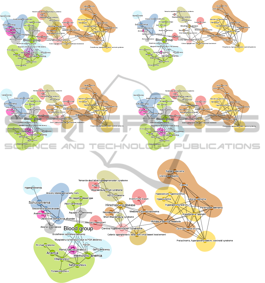
(a) (b)
(c) (d)
(e)
Figure 10: A part of the human disease network (Goh et al., 2007). Case (a) is recreated from the diseasome poster available
at http://diseasome.eu/poster.html and uses a Gaussian distribution function with no negative weights. In this case there are
many unnecessary region overlaps. Cases (b) and (c) show the Gaussian distribution function with negative weights. In (b),
we tried to preserve the blobbiness of the shapes in (a), however this results in some regions disappearing completely. In (c)
this is remedied at the cost of the blobbiness of the regions. Cases (d) and (e) show the results of the proposed method. (d)
closely resembles the results of the Gaussian function in (c). However, (e) combines the smooth regions of (a) with correct
overlaps, a result not achievable using a Gaussian function.
the Gaussian in this example. We were also interested
in improving the visualization performed by Mathieu
Bastian and S
´
ebastien Heymann from Gephi (avail-
able online at http://diseasome.eu/poster.html).
AnInverseDistance-basedPotentialFieldFunctionforOverlappingPointSetVisualization
37

5 CONCLUSIONS
We presented a new potential field function for over-
lapping point set visualization in the form of Euler di-
agrams. In contrast to the most widely used potential
functions, the proposed function ensures correct point
membership in the set regions. Moreover, it retains all
desired Gaussian-based potential field function prop-
erties, e.g., the set region shapes are smooth and vi-
sually pleasing. Set regions are easily identifiable and
closely match the layout of the points. The smooth-
ness and size of the regions can be also adjusted using
the parameters of our function.
We have applied our function on different real-
world examples and compared the result to the ear-
lier methods. The proposed function is very effective
in cases with no intersecting sets, since then the re-
gions are guaranteed not to overlap. It also works
well with overlapping sets, with regions creating an
easily comprehensible Euler diagram, retaining cor-
rect point membership. We have demonstrated that
our function works well in cases where it is not possi-
ble to obtain a good result using the Gaussian poten-
tial function. We have also illustrated how the overall
approach can be successfully used to visualize over-
lapping graph clustering.
REFERENCES
Balzer, M. and Deussen, O. (2007). Level-of-detail visual-
ization of clustered graph layouts. 2007 6th Interna-
tional AsiaPacific Symposium on Visualization, pages
133–140.
Blinn, J. F. (1982). A generalization of algebraic surface
drawing. ACM Trans. Graph., 1(3):235–256.
Byelas, H. and Telea, A. (2009). Towards realism in draw-
ing areas of interest on architecture diagrams. Journal
of Visual Languages Computing, 20(2):110–128.
Collins, C., Penn, G., and Carpendale, S. (2009). Bubble
sets: Revealing set relations with isocontours over ex-
isting visualizations. IEEE Transactions on Visualiza-
tion and Computer Graphics, 15(6):1009–1016.
Di Battista, G., Eades, P., Tamassia, R., and Tollis, I. G.
(1998). Graph Drawing: Algorithms for the Visual-
ization of Graphs. Prentice Hall PTR.
Dinkla, K., van Kreveld, M. J., Speckmann, B., and West-
enberg, M. A. (2012). Kelp diagrams: Point set mem-
bership visualization. Computer Graphics Forum,
31(3pt1):875–884.
Douglas, D. H. and Peucker, T. K. (1973). Algorithms for
the reduction of the number of points required to rep-
resent a digitized line or its caricature. Cartograph-
ica The International Journal for Geographic Infor-
mation and Geovisualization, 10(2):112–122.
Gansner, E. R., Hu, Y., and Kobourov, S. (2010). GMap: Vi-
sualizing graphs and clusters as maps. 2010 IEEE Pa-
cific Visualization Symposium PacificVis, pages 201–
208.
Goh, K.-I., Cusick, M. E., Valle, D., Childs, B., Vidal, M.,
and Barabsi, A.-L. (2007). The human disease net-
work. Proceedings of the National Academy of Sci-
ences of the United States of America, 104(21):8685–
8690.
Gross, M. H., Sprenger, T. C., and Finger, J. (1997). Vi-
sualizing information on a sphere. In In Proceedings
of the 1997 Conference on Information Visualization,
pages 11–16.
Heer, J. and Boyd, D. (2003). Vizster: visualizing online
social networks. IEEE Symposium on Information Vi-
sualization 2005 INFOVIS 2005, 5(page5):32–39.
Hobby, J. D. (1986). Smooth, easy to compute interpolat-
ing splines. Discrete and Computational Geometry,
1(2):123–140.
Krebs, V. (2007). Managing the 21st century organization.
IHRIM Journal, XI(4):2–8.
Matsumoto, Y., Umano, M., and Inuiguchi, M. (2008). Vi-
sualization with Voronoi tessellation and moving out-
put units in self-organizing map of the real-number
system. Neural Networks, 1:3428–3434.
Riche, N. H. and Dwyer, T. (2010). Untangling Euler dia-
grams. IEEE Transactions on Visualization and Com-
puter Graphics, 16(6):1090–1099.
Rosenthal, P. and Linsen, L. (2009). Enclosing surfaces
for point clusters using 3D discrete Voronoi diagrams.
Computer Graphics Forum, 28(3):999–1006.
Santamara, R. and Thern, R. (2008). Overlapping clustered
graphs: Co-authorship networks visualization. Lec-
ture Notes in Computer Science, 5166:190—199.
Simonetto, P., Auber, D., and Archambault, D. (2009).
Fully automatic visualisation of overlapping sets.
Computer Graphics Forum, 28(3):967–974.
Sprenger, T. C., Brunella, R., and Gross, M. H. (2000). H-
BLOB: a hierarchical visual clustering method using
implicit surfaces. In Visualization 2000. Proceedings,
pages 61 –68.
Van Ham, F. and Van Wijk, J. J. (2004). Interactive visu-
alization of small world graphs. IEEE Symposium on
Information Visualization, pages 199–206.
Watanabe, N., Washida, M., and Igarashi, T. (2007). Bub-
ble clusters: an interface for manipulating spatial ag-
gregation of graphical objects. In Proceedings of the
20th annual ACM symposium on User interface soft-
ware and technology, UIST ’07, pages 173–182, New
York, NY, USA. ACM.
IVAPP2014-InternationalConferenceonInformationVisualizationTheoryandApplications
38
