
A Practical and Robust Method to Compute the Boundary of
Three-dimensional Axis-aligned Boxes
Daniel L
´
opez Monterde, Jon
`
as Mart
´
ınez, Marc Vigo and N
´
uria Pla
Departament de Llenguatges i Sistemes Inform
`
atics, Universitat Polit
`
ecnica de Catalunya, Edifici ETSEIB, Diagonal 647,
8a Planta E, 08028 Barcelona, Spain
Keywords:
Boundary representation, Union of boxes, Orthogonal polyhedra.
Abstract:
The union of axis-aligned boxes results in a constrained structure that is advantageous for solving certain
geometrical problems. A widely used scheme for solid modelling systems is the boundary representation (B-
rep). We present a method to obtain the B-rep of a union of axis-aligned boxes. Our method computes all
boundary vertices, and additional information for each vertex that allows us to apply already existing methods
to extract the B-rep. It is based on dividing the three-dimensional problem into two-dimensional boundary
computations and combining their results. The method can deal with all geometrical degeneracies that may
arise. Experimental results prove that our approach outperforms existing general methods, both in efficiency
and robustness.
1 INTRODUCTION
Many of the current solid modelling systems are
based on Boundary Representations (B-rep) and Con-
structive Solid Geometry (CSG). Computing the B-
rep of the resulting solid of CSG, after performing
boolean operations, is a fundamental operation in
these systems. The problem of robust and accurate
computation of the boundary is considered one of
the difficult problems in solid modelling (Hoffmann,
1996). Most of the effort in the subject is focused
on boolean operations between polyhedral or alge-
braic objects (Requicha and Voelcker, 1985; Thibault
and Naylor, 1987). The restricted case of three-
dimensional axis-aligned boxes has received less in-
terest, even though its bounded structure can lead
to robust and simple algorithms. Furthermore, the
union of axis-aligned boxes is an orthogonal poly-
hedron. Their constrained structure has enabled ad-
vances on complex or unsolved problems for arbitrary
shapes (Bournez et al., 1999; Vigo et al., 2012).
Orthogonal polyhedra have been directly stud-
ied for mesh reconstruction from scanner data (Biedl
et al., 2009) and urban modelling (Sugihara and
Hayashi, 2008). They have also been used to bound or
approximate more complex shapes, with applications
in spatial databases (Esperanc¸a and Samet, 1997), and
motion planning (Albers et al., 1999). In particular, an
efficient algorithm that obtains the union of boxes is
required to compute the skeleton of orthogonal poly-
hedra (Martinez et al., 2013)
The problem of computing the two-dimensional
boundary of the union of a set of axis-aligned rectan-
gles, among other properties, sparked interest in the
1980s (Jr. and Preparata, 1980; Wood, 1984; G
¨
uting,
1984). Several methods were proposed, and the prob-
lem has been optimally solved since then. Its exten-
sion to three dimensions, however, has received little
attention in the literature.
Our aim is to fill that gap, by presenting an algo-
rithm that computes the boundary of the union of a
set of axis-aligned three-dimensional boxes. The out-
put of the presented method is a B-rep of the union of
the boxes. For this purpose, we apply the results pre-
sented by Vigo et al. (Vigo et al., 2012). Their algo-
rithm obtains the B-rep from the list of vertices in an
orthogonal polyhedron’s boundary and additional in-
formation concerning the local topology of each ver-
tex. Our computes this information in order to apply
Vigo et al.’s algorithm and obtain a B-rep.
Our approach consists in dividing the overall com-
putation into a series of 2D boundary computations,
and then combining their results to obtain the 3D
boundary. The obtained results demonstrate that the
robustness of the 2D computation, which is much eas-
ier to obtain, directly implies the robustness in the
three-dimensional case. Our method makes use of an
axis-aligned plane, which is swept through the set of
34
López Monterde D., Martínez J., Vigo M. and Pla N..
A Practical and Robust Method to Compute the Boundary of Three-dimensional Axis-aligned Boxes.
DOI: 10.5220/0004682800340042
In Proceedings of the 9th International Conference on Computer Graphics Theory and Applications (GRAPP-2014), pages 34-42
ISBN: 978-989-758-002-4
Copyright
c
2014 SCITEPRESS (Science and Technology Publications, Lda.)

boxes. The plane is positioned between all pairs of
consecutive faces, its intersection with the boxes in-
ducing a set of rectangles. The 2D boundary of the
set of rectangles is computed using already existing
methods. Then, the final 3D boundary is obtained by
comparing consecutive 2D boundaries.
One of the most challenging aspects of geometri-
cal algorithms is to achieve robustness, given the vari-
ety of possible inputs (Hoffmann, 1989). Even when
the domain is restricted to axis-aligned polyhedra, de-
generate cases can still pose a problem. A geometrical
degeneracy can be caused by the existance of copla-
nar faces, colinear edges, or coincident vertices. Non-
trihedral vertices can also be considered degeneracies,
and they can be originated from the previously men-
tioned degeneracy kinds.
Our method is robust to all cases, and it generates
the expected output for any given input. It is able to
handle floating point numbers, and, most importantly,
generates no underflow conditions, by applying only
comparison and assignation operators on them.
Besides its robustness, our algorithm has other
noteworthy positive properties. Additionally, it re-
quires no complex data structures to be implemented.
Due to separating 3D from 2D concerns, the method
is highly parallelizable.
2 RELATED WORK
The properties of union hyper-rectangles have been
the focus of theoretical study. It is known that the
union of n axis-aligned boxes in dimension d has a
worst-case combinatorial complexity of θ
n
d
. If the
boxes are hypercubes, the union has combinatorial
complexity of O
n
dd/2e
. If the hypercubes have con-
stant size the complexity reduces to O
n
bd/2c
(Bois-
sonnat et al., 1998). Kaplan et al. presented an
algorithm to compute the union of d-dimensional
hypercubes of constant size in O
n
bd/2c
polylog n
time (Kaplan et al., 2007).
In the literature, most of the effort is devoted to
compute the volume of the union, which is known as
Klee’s measure problem (Klee, 1977), rather than ex-
plicitly constructing the union. Interestingly, when
d > 2 the volume can be computed more efficiently
than the union. For example, the algorithm of Over-
mars and Yap runs in O
n
d/2
logn
time (Overmars
and Yap, 1991). It remains an open question whether
faster algorithms are possible, or if it is possible to
prove tighter lower bounds. In particular, it remains
open whether the algorithm’s running time must de-
pend on d (Chan, 2010). Unfortunately, as the worst-
case complexity of the union of axis aligned boxes is
θ
n
d
, theoretical efforts have been focused on the
efficient computation of their volume.
Two different main strategies were proposed to
compute the union of two-dimensional axis-aligned
rectangles: sweep line (Jr. and Preparata, 1980) and
divide and conquer (G
¨
uting, 1984) algorithms. Both
algorithm types run in O (n log n + k) time, where k is
the number of vertices of the union.
Concerning the three-dimensional case, there ex-
ist several classical methods to compute the boundary
of CSG (Requicha and Voelcker, 1985). Most of them
classify the set of CSG primitives with some kind of
spatial decomposition scheme (Thibault and Naylor,
1987). Hachenberger et al. have studied and opti-
mized boolean operations on Nef Polyhedra, and that
handle all cases, including all degeneracies (Hachen-
berger and Kettner, 2005). Baumann et al. compute
the union of three dimensional axis-aligned boxes,
represented by a set of enclosing rectangles, by an
octree-based incremental algorithm (Baumann et al.,
2008). Campen et al. presented a robust method
that computes boolean operations using an adaptive
octree with nested binary space partitions (Campen
and Kobbelt, 2010). Schifko et al. presented a robust
sweeping plane algorithm to compute boolean oper-
ations on meshes, based on R-trees (Schifko et al.,
2010).
3 PREVIOUS DEFINITIONS
In this section we introduce some basic definitions
used throghout the paper.
A polygon is a bounded subset of R
2
enclosed by a
finite set of line segments, called edges. The edges
meet only at their endpoints, called vertices. A
polygon face is a single connected component of
a polygon.
An orthogonal polygon is a polygon enclosed by
axis-aligned edges. An edge is called vertical if
it is parallel to the ordinate and horizontal if it is
parallel to the abscissa.
An orthogonal manifold polygon is an orthogonal
polygon such that every vertex is shared by a ver-
tical and a horizontal edge.
An orthogonal pseudomanifold polygon is a general-
ization of an orthogonal manifold polygon, which
allows non-manifold vertices. A non-manifold
vertex is a vertex polygon with four incident
edges.
A polyhedron is a bounded subset of R
3
enclosed
by a finite set of non-intersecting planar polygons,
called faces.
APracticalandRobustMethodtoComputetheBoundaryofThree-dimensionalAxis-alignedBoxes
35
+X
+Y
+Z
(a) (b) (c) (d) (e)
(j)(i)(h)(g)(f)
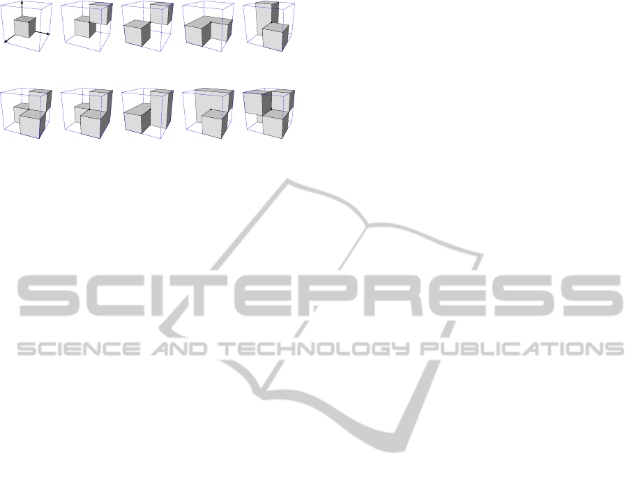
(1,0,1,0,1,0) (2,0,1,1,1,1) (1,1,1,1,1,1) (1,0,1,0,1,0) (0,1,0,1,1,0)
(2,1,1,2,2,1) (2,0,0,2,2,0) (2,0,1,1,2,0) (1,1,1,1,1,1) (2,2,2,2,2,2)
Figure 1: Possible vertex configurations of an orthogonal
pseudomanifold polyhedron. The six numbers below each
configuration correspond to the face degrees that must be
generated for them (+x,−x,+y,−y,+z,−z).
A trihedral vertex is a vertex of a polyhedron that
has exactly three incident faces.
An orthogonal polyhedron is a polyhedron enclosed
by axis-aligned faces.
An orthogonal manifold polyhedron is an orthogo-
nal polyhedron such that every edge of a face is
shared by exactly one other face.
An orthogonal pseudomanifold polyhedron is a gen-
eralization of an orthogonal manifold polyhedron,
which allows non-manifold edges or vertices. A
non-manifold edge is an edge adjacent to four
faces and a non-manifold vertex is a non-trihedral
vertex.
A boundary representation model (B-rep) repre-
sents a shape by a collection of its boundary ele-
ments and their topological relationships. Bound-
ary representation models are composed of two
parts: geometry (surfaces, curves and points) and
topology. The main topological items are faces,
edges and vertices. A face is a bounded portion of
a surface; an edge is a bounded piece of a curve
and a vertex lies at a point. The topological in-
formation defines the relationship among the geo-
metric elements.
4 VERTEX CONFIGURATIONS
In this section, we define the additional information
that needs to be computed for every boundary ver-
tex. This information encodes the local topology of
the vertex (see Figure 1) and it is required to prevent
ambiguity in the reconstruction. It is the input needed,
in addition to the vertex coordinates, for the B-rep
extraction by Vigo et al. (Vigo et al., 2012). There
are ten basic local configurations for a vertex. All
the other possible configurations can be derived from
these by considering only rotation and complement
operations (Aguilera, 1998).
Each possible configuration requires specific in-
formation to be computed (see Figure 1). This cor-
responds to the number of different faces converging
at the vertex that are oriented in each of the six or-
thogonal directions (+x, −x, +y,−y,+z,−z). For this
reason, we refer to this information as vertex face de-
grees. There is one special case, (h), in which ex-
actly four different faces intersect at the vertex. This
configuration requires an exception to be made to the
general rule. In this case, for the B-rep reconstruction
to work, the two non-coplanar faces intersecting at the
vertex have to be counted twice.
Our approach for computing the vertex face de-
grees is based on the following observations:
• Trihedral vertices, such as the one in (a), have a
total face degree of three, one for each axis.
• The rest of the vertex configurations can be ob-
tained by considering them as a combination of a
number of trihedral vertices.
Cases (d) and (e), as well as (a), can be obtained
with a single trihedral vertex. Cases (b, c, g,h,i) can
be obtained by combining the face degrees of two ver-
tices. Case ( f ) needs the combination of three ver-
tices, and case ( j) needs to combine four trihedral
vertices (see Figure 1).
These observations allow us to design our method
so that it obtains only trihedral vertices. For the con-
figurations where more than one vertex is needed to
form the vertex face degrees, the method obtains each
trihedral vertex independently. It is easily seen that it
is possible to decompose all configurations into spe-
cific trihedral vertices, the degrees of which can be
combined into the required ones. After all trihedral
vertices are computed, those sharing the same coordi-
nates are merged into a single vertex. That vertex has
as its face degrees the sum of the face degrees of all
the vertices that shared its coordinates.
5 TWO-DIMENSIONAL
BOUNDARY EXTRACTION
Input Set of axis-aligned rectangles
Output Set of vertices that form the boundary of the
union of the input rectangles, and the x and y di-
rections of each vertex
Each 2D boundary is computed by the time-optimal
method described by G
¨
uting (G
¨
uting, 1984). The
method takes a set of axis aligned rectangles as its
GRAPP2014-InternationalConferenceonComputerGraphicsTheoryandApplications
36
(a)
y
x
(b)
y
x
stripe
x-interval
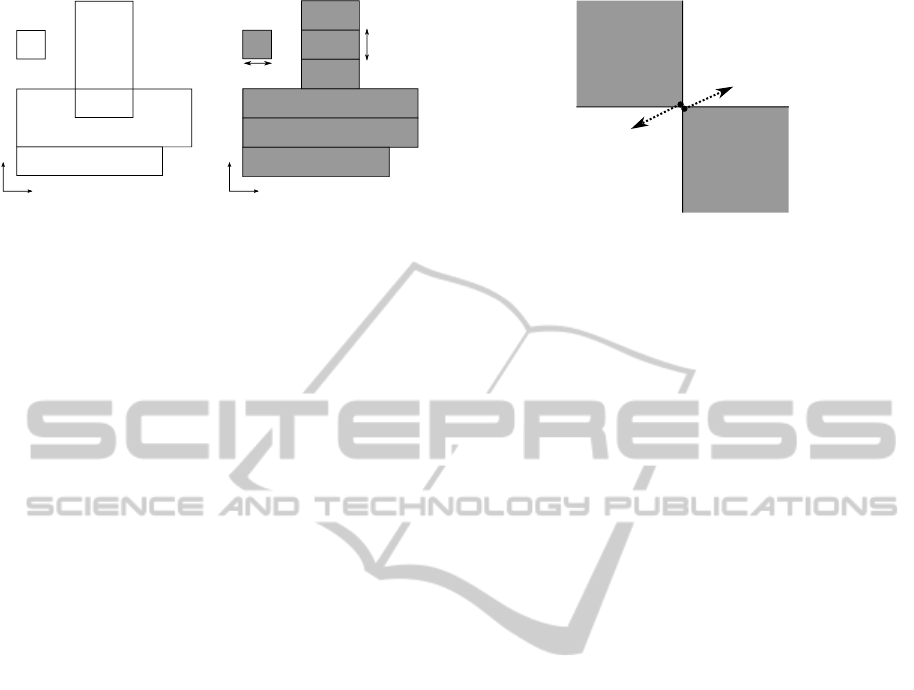
Figure 2: (a) Original set of rectangles. (b) Representation
obtained after the first step.
input, and obtains the list of all edges in the bound-
ary of their union. However, it does not distinguish
the edges that define external boundaries from those
which define polygon holes. The method is divided
in two steps. In the first step, it computes a repre-
sentation of the union. In the second, it uses the ob-
tained representation to compute the boundary edges.
Because we require additional information for every
vertex, we extend the second step of the algorithm.
The first step uses a divide and conquer approach.
Each rectangle is represented by its two vertical
edges: a technique G
¨
uting calls separational repre-
sentation. The representation obtained (shown in Fig-
ure 2(b)) is a set of horizontal stripes spanning the
polygon that constitutes the union. Each stripe con-
tains a binary tree with the x-intervals where it is vis-
ible.
In the second step, the obtained representation is
used to compute the boundary. Each horizontal edge
in the input set of rectangles is considered. It is
matched to one of its adjacent stripes, which is the
stripe above it if the edge is top and the stripe below it
if it is bottom. The tree of x-intervals associated with
the stripe is queried with the x-interval corresponding
to the edge. The leaves in the tree that are within the
edge’s interval represent boundaries of the polygon,
and are therefore vertices of the boundary.
At this point, all horizontal edges have been com-
puted, so we have all the vertices in the boundary.
5.1 Vertex Face Degree Computation
We have to adapt the algorithm so that it generates
the information needed for the B-rep extraction. Hav-
ing already shown how the vertices of the boundary
are obtained, we consider the problem of generating
the face degrees for each of them. During the second
step of the 2D computation, we obtain the vertex face
degrees in the x and y axes.
The x face degrees indicate whether the orienta-
tion of face that generated the vertex in this 2D bound-
(1,0,0,1)
(0,1,1,0)
Figure 3: A non-manifold vertex in two dimensions, and its
decomposition in two vertices. The numbers indicate the
face degrees for each vertex, in (+x,−x,+y,−y) format.
ary was right (+x) or left (−x). To compute them, we
need to know what side of the x-interval the vertex
was obtained from. If it was left end, the −x degree
of the vertex is 1, and the +x degree is 0. And vicev-
ersa, +x = 1 and −x = 0, if it was the right end.
Analogously, the y degrees indicate whether the
face that generated the vertex was facing top (+y) or
bottom (−y). They can be computed in a straightfor-
ward way. In this case, we need to know if the edge
they were obtained from was a top or a bottom edge.
For the top edges, we have 1 in the +y degree and 0
in the −y; and viceversa for bottom edges.
Trying to apply the above principles to non-
manifold vertices leads us to ambiguity. This is due
to the fact that non-manifold vertices in two dimen-
sions are intersected by four segments (see Figure 3).
These vertices appear when two different rectangles
have opposite vertices in the same space coordinates.
Our method for dealing with non-manifold vertices
consists of considering them a combination of two in-
dependent vertices. This leaves us with two vertices
in the same coordinates, pointing at opposed direc-
tions (see Figure 3). Each of them generates a tri-
hedral vertex when extended to the third dimension,
fulfilling the observations in Section 4. As we already
mentioned, the resulting face degrees for that vertex
are obtained from the sum of the trihedral vertices
sharing the same coordinates.
6 THREE-DIMENSIONAL
BOUNDARY EXTRACTION
Input Set of axis-aligned boxes
Output Set of vertices that constitute the boundary
of the union of the input boxes, and the x, y and z
degree of each vertex
The algorithm follows a two step structure. In the first
step, the set of boxes is divided into distinct 2D slices,
APracticalandRobustMethodtoComputetheBoundaryofThree-dimensionalAxis-alignedBoxes
37
⊕ ⊕ ⊕ ⊕ ⊕ ⊕
x
y
z
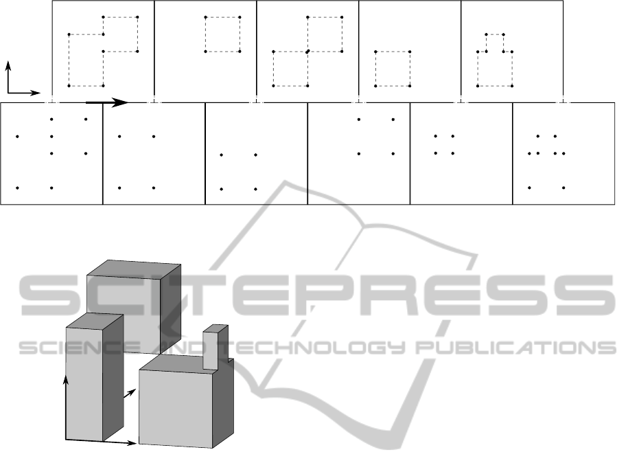
Figure 5: The top part of the figure shows the slices generated from the boxes in Figure 4. The bottom part shows the result
of the vertex-wise xor merge. Each of the squares in the bottom corresponds to the xor of the two squares above it.
z
x
y
Figure 4: Visualization of the union of a set of four boxes.
and the 2D boundary of each slice is computed by the
method defined in Section 5. In the second step, the
obtained 2D boundaries are sequentially compared to
obtain the orthogonal polyhedron that constitutes the
3D boundary.
For the first step, we consider a plane perpendicu-
lar to the z axis that advances through the boxes. The
intersection of the plane with the boxes induces a 2D
slice, formed by a set of rectangles. We have to decide
in what positions of the plane the 2D slices are com-
puted. The key idea is that a vertex is in the 3D bound-
ary if it changes between consecutive slices, that is, if
the vertex appears in one slice but not in the other.
Thus, we consider slices right after each unique z co-
ordinate in the set of boxes. In this manner, the ver-
tices that appear in the boundaries of the slices repre-
sent the topology of the 3D boundary at every point
in which it changes. As a consequence, local changes
between two consecutive slices can be used to obtain
the vertices of the 3D boundary. A perspective visu-
alization of a set of boxes (Figure 4) and the slices
obtained from it (top part of Figure 5) are shown as
an example.
Analogously to the 2D algorithm, separational
representation is used for the boxes. They are rep-
resented by their two z-faces, which we refer to as
front if they are oriented towards +z, and back if they
are oriented towards −z. The faces are sorted by z,
with back faces going before front ones with the same
z, and the z-plane is swept over them. We represent
the induced slice as a list of rectangles. To mantain it,
when a back face intersects the plane, it is added to the
list, and when a front face intersects it, the back face
belonging to the same box is removed. After each
face is added, we check if the next face in the list has
a different z. In that case, the 2D boundary of the cur-
rent state of the slice is computed. Since it is possible
for a vertex to be generated from the intersection of
two faces on the same z, one of which is back and the
other is front, we also generate the boundary of the
slice if the last processed face is back and the next
face to process is front. The first step ends when all
the faces are processed.
In the second step, the 3D boundary is constructed
by a merge algorithm. The vertex-wise xor between
each pair of consecutive slices is computed (see Fig-
ure 5). All vertices that appear in one slice, but not in
both, are in the 3D boundary. When one such vertex
is found, its z-coordinate is set as the previous slice’s
z.
The xor merge is done by advancing in parallel in
the two slices. It is necessary to define a strict weak
ordering between vertices. The vertices in each slice
must be sorted by this ordering. Then, starting by the
first vertex on each slice, they are compared. If they
are equal, they’re not part of the xor, so one element
is advanced in both lists. If they are different, we ad-
vance an element on the list that had the smaller ele-
ment, and that element is added as a vertex. This way
we can compute which vertices are in one slice but
not the other in linear time respect to the number of
GRAPP2014-InternationalConferenceonComputerGraphicsTheoryandApplications
38

vertices.
It is worth noting that the algorithm does not re-
quire complex data structures. Only basic sequence
containers, such as arrays, are required.
The presented algorithm also has the advantage of
being independent of the 2D algorithm chosen, pro-
vided the 2D algorithm generates the necessary out-
put. This output consists only of the vertices and their
face degrees in x and y, which should be computable
straightforwardly.
6.1 Vertex Face Degree Computation
During the xor merge, we compute the z face degrees
of each vertex. We need the output to be exactly like
the one we defined in section 4, so we have to take
a close look at each of the possible configurations.
To differentiate them, it is necessary to know where
a vertex is, regarding the adjacent boundary.
A 3D vertex can be found in two manners: by
comparison with the 2D boundary in front of it or
by comparison with the boundary behind. Indepen-
dently of that classification, it can also be, regarding
the adjacent boundary, inside it or outside it. It is pos-
sible that a vertex is exactly in the boundary, and in
this case it is classified as either inside or outside and
treated accordingly.
If a vertex is outside the adjacent boundary, only
the boundary in which the vertex was found has to
be considered. Thus, outside front vertices look at
+z, and outside back vertices at −z. Vertices that are
inside follow the same reasoning: Only the adjacent
boundary is considered for the face degree, so inside
front vertices look at −z and inside back vertices at
+z.
To determine the classification for vertices that are
in an edge of the adjacent boundary, we need to look
at the already computed x and y face degrees. We
have to consider that an edge has only one significant
direction, which is x for vertical edges, and y for hor-
izontal ones. If an edge shares its direction with the
corresponding direction of the vertex, it means they
split the space in the same way. Thus, a vertex that
coincides with an edge is classified to be inside if and
only if they face the same direction.
6.2 Algorithm
A pseudocode overview of the algorithm is shown
(see Algorithm 1). We explain some of the notation
used.
The faces have a z coordinate, and the direction
they face is indicated. For a given face f , these are
noted as f .z and f . f ront, respectively.
We consider each vertex to be defined by its coor-
dinates and face degrees in the applicable dimensions.
For a given vertex v, these are noted as v.x, v.y, v.z and
v. f ace degrees.
We use ⊕ to denote the vertex-wise merge xor we
defined in Section 6. It should be noted that it com-
putes the z face degree for all resulting vertices.
For brevity, we denote the next element e in a con-
tainer as next(e).
Algorithm 1: 3D boundary.
INPUT: Set of axis-aligned boxes B
Set of active z-faces F ←
/
0
for all box b in B do
F ← F ∪ f ront f ace(b)
F ← F ∪ back f ace(b)
end for
sort(F) {faces are sorted in z, then front}
Vector of 2D Boundary V 2DB ←
/
0
Current slice S ←
/
0
for all face f in F do
if f is back then
S ← S ∪ f
else
S ← S \ face matching f
end if
if f .z 6= next( f ).z ∨ ( f . f ront ⊕ next( f ). f ront)
then
V 2DB ← V 2DB ∪ 2D Boundary(S)
end if
end for
Set of boundary vertices V ←
/
0
for i ← 1..size(V 2DB) − 1 do
V ← V ∪V2DB[i] ⊕V 2DB[i + 1]
end for
for i ← 1..size(V ) − 1 do
if V [i].x = V [i + 1].x ∧ V [i].y = V [i + 1].y ∧
V [i].z = V [i + 1].z then
V [i]. f ace degrees ← V [i]. f ace degrees +
V [i + 1]. f ace degrees
V ← V \V[i]
end if
end for
OUTPUT: Set of vertices V
7 RESULTS
The presented method has been implemented in C++.
It should be noted that for the two-dimensional
boundary computation, G
¨
uting’s method is not used.
A simpler method was implemented for the 2D
boundary computation, with a theoretical time com-
plexity of O(n
2
), instead of O(nlogn + k). This
APracticalandRobustMethodtoComputetheBoundaryofThree-dimensionalAxis-alignedBoxes
39
0
10
20
30
40
50
60
70
80
0 1000 2000 3000 4000 5000 6000
Time (s)
Boxes
d = 0.02 n
d = 0.05 n
7
5
d = 0.1 n
9
5
d = 0.3 n
11
5
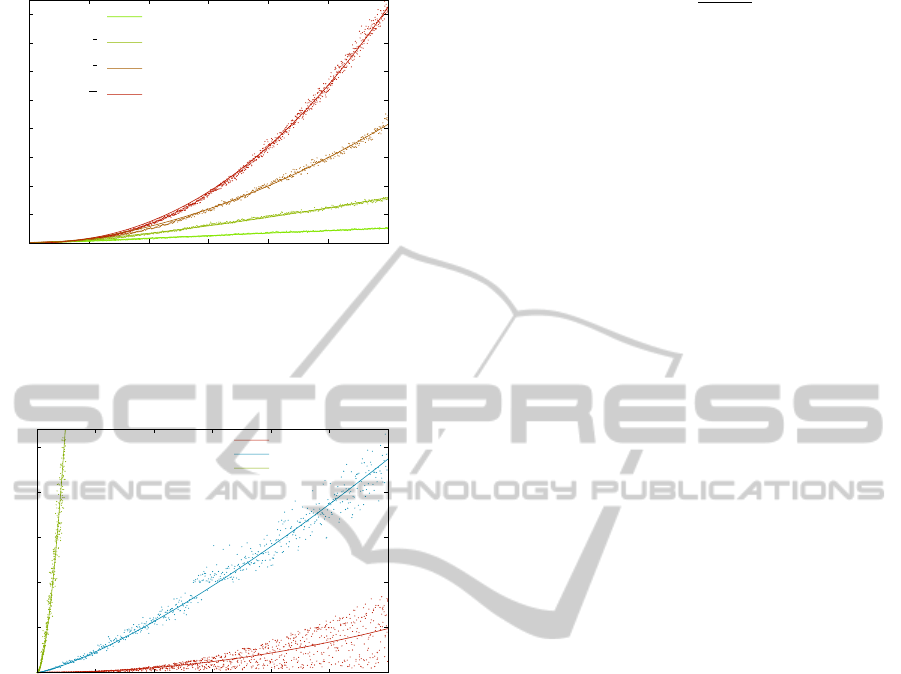
Figure 6: Running times of the presented method to com-
pute the B-rep of several boxes with varying densities. Ev-
ery point depicts the runtime for a single dataset. Every line
corresponds to the curve fitted to average runtime of each
density, with respect to the number of boxes.
0
50
100
150
200
250
0 1000 2000 3000 4000 5000 6000
Time (s)
Boxes
Our method
CARVE
CGAL
Figure 7: Running times of CARVE to compute the B-rep
of several sets of boxes. The plot follows the same scheme
of Figure 6.
means that the presented experimental results have
room for improvement in the efficiency area. The
source code consists of about 800 lines of code, half
of them correspond to the two-dimensional bound-
ary computation, and the remaining ones to the three-
dimensional part. The B-rep extraction is performed
using its publically available Python implementa-
tion (Vigo, 2011).
All the presented results were performed on PC
i7-3770 clocked at 3.9GHz core and 16 GB of RAM
memory.
Figure 6 shows the results for over 30000 ran-
dom cases with varying density of boxes. The den-
sity measures the average number of rectangles pro-
cessed in each slice. The minimum amount, 1 rectan-
gle per slice, corresponds to the value 0. The maxi-
mum amount, n rectangles in each slice, corresponds
to 1. The value increases linearly between both ex-
tremes. The formula used is
nr/2−n
2
n
3
−n
2
, where n is the
number of boxes and r the total of boxes processed in
all slices.
We compared our approach with CGAL and
CARVE. We used CGAL’s implementation of
Nef Polyhedra with an arbitrary precision kernel
(Gmpz) (CGAL, 2013). CARVE is a robust octree-
based constructive solid geometry library (Sargeant,
2013).
Figure 7 shows a comparison of the running time
of our method with the other methods, all with ran-
dom densities. The computation times of our method
include the B-rep computation from the boundary ver-
tices. We observed that the running time of our algo-
rithm is highly correlated with the box density, that
is, the average number of rectangles contained in each
slice. Thus, it can be seen experimentally that our al-
gorithm is not output-sensitive. It should be noted that
none of the randomly generated cases had a density
over 0.35. This implies that inputs approaching the
worst case, with densities close to 1, are extremely
rare and do not occur naturally. On average, the run-
time performance of the presented approach is of the
order O(n
7/5
), where n is the number of boxes, which
coincides with the one obtained by CARVE. CGAL’s
experimental running time can be fitted to O(n
9/5
).
Unfortunately, CARVE was unable to terminate
the execution for some degenerate inputs, constitut-
ing 13% of the total of datasets. Even for the datasets
where it terminated, the generated output was in some
instances incorrect. Due to the difficulty of automati-
cally checking the correctness of the CARVE output,
we can not estimate the amount those represent. The
mentioned errors were detected via manual verifica-
tion of the output.
8 CONCLUSION AND FUTURE
WORK
A method was presented to compute the boundary of
the union of a set of axis-aligned boxes. It divides
the computation of the 3D boundary into a series of
2D boundary computations, and then combines their
results.
As shown in Section 7, the presented method ex-
hibits lower experimental running time than previous
existing general methods, such as CARVE and CGAL
(Figure 7). More importantly, it deals with all degen-
erate cases, generating the correct B-rep in 100% of
the cases. It significantly outperforms CARVE in this
regard too, since CARVE failed to terminate in 13%
of cases, and obtained incorrect results in others.
GRAPP2014-InternationalConferenceonComputerGraphicsTheoryandApplications
40
(a) (b)
(c) (d)
(e) (f)
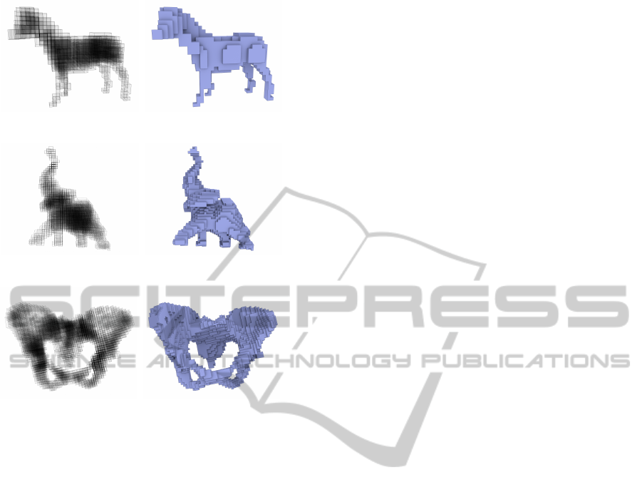
Figure 8: (a,c,e) Set of boxes obtained from voxel models
of a horse, an elephant and a human pelvis. Darker shades
indicate higher density of boxes. (b, d, f) Visualization of
the B-rep obtained with our method each respective input.
The method is independent from the 2D imple-
mentation, thus any method for computing the 2D
boundary can be used. Interestingly, due to its struc-
ture, it allows for parallelization, since in the first step,
each call to the 2D boundary method is independent
from all others. Furthermore, each xor merge in the
second step is also independent, so there is also po-
tential for parallelization in that area.
With the presented method, each 2D boundary is
computed independently, when in practice many of
the rectangles are shared by adjacent boundaries. This
implies that our method potentially performs dupli-
cated computations. The challenge remains to design
a dynamic data structure for the boundary of the union
of rectangles. Such a data structure would need to
keep a representation of the 2D boundary, and pro-
vide efficient operations to insert and delete rectan-
gles from it. With it, the duplicated computations
that result from treating each 2D slice independently
would not be necessary, which would reduce the run-
ning time. However, it would lose the independence
from the 2D boundary computation, so it would not
be easily parallelizable.
The described method only considers the union
operation on the set of boxes. However, it would
be interesting to consider other boolean operations in
which the method could be applied, most notably the
intersection. It is possible that our method can be
straightforwardly extended to deal with these opera-
tions, but careful analysis would be required.
The implementation is available at http://
lafarga.cpl.upc.edu/projectes/boxunion3d
under the GPL license. By doing that, we aim to
make it possible for other researchers to use it, as
well as contribute to it or modify it.
ACKNOWLEDGEMENTS
This work has been partially supported by the project
TIN2008-02903 and TIN2011-24220 of the Spanish
government and by the IBEC (Bioengineering Insti-
tute of Catalonia).
REFERENCES
Aguilera, A. (1998). Orthogonal Polyhedra: Study and
Application. PhD thesis, Universitat Polit
`
ecnica de
Catalunya.
Albers, S., Kursawe, K., and Schuierer, S. (1999). Explor-
ing unknown environments with obstacles. In Pro-
ceedings of the tenth annual ACM-SIAM symposium
on Discrete algorithms, pages 842–843.
Baumann, T., Jans, M., Sch
¨
omer, E., Schweikert, C., and
Wolpert, N. (2008). Dynamic free-space detection for
packing algorithms. In EuroCG’08, pages 43–46.
Biedl, T., Durocher, S., and Snoeyink, J. (2009). Recon-
structing polygons from scanner data. Lecture Notes
in Computer Science, 5878:862–871.
Boissonnat, J.-D., Sharir, M., Tagansky, B., and Yvinec, M.
(1998). Voronoi diagrams in higher dimensions under
certain polyhedral distance functions. Discrete and
Computational Geometry, 19(4):485–519.
Bournez, O., Maler, O., and Pnueli, A. (1999). Orthogonal
polyhedra: Representation and computation. Lecture
Notes in Computer Science, 1569:46–60.
Campen, M. and Kobbelt, L. (2010). Exact and robust
(self-) intersections for polygonal meshes. Computer
Graphics Forum, 29:397–406.
CGAL (2013). CGAL, Computational Geometry Algo-
rithms Library. http://www.cgal.org.
Chan, T. M. (2010). A (slightly) faster algorithm for
Klee’s measure problem. Computational Geometry,
43(3):243–250.
Esperanc¸a, C. and Samet, H. (1997). Orthogonal polygons
as bounding structures in filter-refine query process-
ing strategies. Lecture Notes in Computer Science,
1262:197–220.
APracticalandRobustMethodtoComputetheBoundaryofThree-dimensionalAxis-alignedBoxes
41

G
¨
uting, R. H. (1984). An optimal contour algorithm for iso-
oriented rectangles. Journal of Algorithms, 5(3):303–
326.
Hachenberger, P. and Kettner, L. (2005). Boolean opera-
tions on 3d selective nef complexes: optimized im-
plementation and experiments. In Proceedings of the
2005 ACM symposium on Solid and physical model-
ing, pages 163–174.
Hoffmann, C. (1989). The problems of accuracy and robust-
ness in geometric computation. Computer, 22(3):31–
39.
Hoffmann, C. (1996). How solid is solid modeling? In
Applied Computational Geometry Towards Geometric
Engineering, volume 1148 of Lecture Notes in Com-
puter Science, pages 1–8. Springer Berlin Heidelberg.
Jr., W. L. and Preparata, F. P. (1980). Finding the contour
of a union of iso-oriented rectangies. Journal of Algo-
rithms, 1(3):235 – 246.
Kaplan, H., Rubin, N., Sharir, M., and Verbin, E. (2007).
Counting colors in boxes. In Proceedings of the eigh-
teenth annual ACM-SIAM symposium on Discrete al-
gorithms, pages 785–794.
Klee, V. (1977). Can the measure of ∪
1
n
[a
i
,b
i
] be computed
in less than O(nlogn) steps? The American Mathe-
matical Monthly, 84(4):284–285.
Martinez, J., Pla-Garcia, N., and Vigo, M. (2013). Skele-
tal representations of orthogonal shapes. Graphical
Models, 75:189–207.
Overmars, M. H. and Yap, C.-K. (1991). New upper bounds
in Klee’s measure problem. SIAM Journal on Comput-
ing, 20:1034—-1045.
Requicha, A. A. G. and Voelcker, H. (1985). Boolean op-
erations in solid modeling: Boundary evaluation and
merging algorithms. Proceedings of the IEEE, 73:30–
44.
Sargeant, T. (2013). Carve. https://code.google.com/
p/carve/.
Schifko, M., J
¨
uttler, B., and Kornberger, B. (2010). In-
dustrial application of exact boolean operations for
meshes. In Proceedings of the 26th Spring Confer-
ence on Computer Graphics, pages 165–172.
Sugihara, K. and Hayashi, Y. (2008). Automatic generation
of 3D building models with multiple roofs. Tsinghua
Science & Technology, 13:368 – 374.
Thibault, W. C. and Naylor, B. F. (1987). Set operations
on polyhedra using binary space partitioning trees. In
Proceedings of the 14th annual conference on Com-
puter graphics and interactive techniques.
Vigo, M. (2011). Orto-brep. http://devel.cpl.upc.
edu/orto-brep/.
Vigo, M., Pla, N., Ayala, D., and Martinez, J. (2012). Ef-
ficient algorithms for boundary extraction of 2D and
3D orthogonal pseudomanifolds. Graphical Models,
74(3):61 – 74.
Wood, D. (1984). The contour problem for rectilinear poly-
gons. Information Processing Letters, 19(5):229–236.
GRAPP2014-InternationalConferenceonComputerGraphicsTheoryandApplications
42
