
Converting Underwater Imaging into Imaging in Air
Tim Dolereit
1,2
and Arjan Kuijper
3
1
Fraunhofer Institute for Computer Graphics Research IGD, Joachim-Jungius-Str. 11, 18059 Rostock, Germany
2
University of Rostock, Institute for Computer Science, Albert-Einstein-Str. 22, 18059 Rostock, Germany
3
Fraunhofer Institute for Computer Graphics Research IGD, Fraunhoferstr. 5, 64283 Darmstadt, Germany
Keywords:
Underwater Image Formation, Underwater Camera Model, Camera Calibration, Underwater Stereo Vision.
Abstract:
The application of imaging devices in underwater environments has become a common practice. Protecting
the camera’s constituent electric parts against water leads to refractive effects emanating from the water-glass-
air transition of light rays. These non-linear distortions can not be modeled by the pinhole camera model. For
our new approach we focus on flat interface systems. By handling refractive effects properly, we are able to
convert the problem to imaging conditions in air. We show that based on the location of virtual object points
in water, virtual parameters of a camera following the pinhole camera model can be computed per image ray.
This enables us to image the same object as if it was situated in air. Our novel approach works for an arbitrary
camera orientation to the refractive interface. We show experimentally that our adopted physical methods can
be used for the computation of 3D object points by a stereo camera system with much higher precision than
with a naive in-situ calibration.
1 INTRODUCTION
The almost standard installation of visual sensors on
autonomous underwater vehicles (AUV) or remotely
operated vehicles (ROV) and the possibility to also
equip divers with them, makes underwater imaging an
efficient sampling tool. Some of the key advantages
of underwater imaging are its non-destructive behav-
ior toward marine life and its repeatable application.
Imaging underwater imposes different constraints
and challenges than imaging in air. One of the main
problems is the refraction of light passing bounding,
transparent interfaces between media with differing
refractive indexes (water-glass-air transition). In this
paper we focus on flat interface systems. Such sys-
tems can be cameras watching through a viewing win-
dow, an aquarium, etc. or cameras inside a special
housing immersed in water. A severe effect induced
during this transition is that objects seem to be closer
to the observer and hence bigger than they actually are
(see figure 1). This refraction induced deviation in di-
mension is dependent on the distance of the imaged
objects to the refractive interface and the incidence
angle of light rays entering the camera through this
interface. This dependency acts in a non-linear way
and poses a problem to every discipline relying upon
metric image information.
Figure 1: left - exemplary magnification and distortion un-
derwater, right - perspective imaging in air.
If it is the task to gain metric information from
the recorded images, the cameras have to be cali-
brated and the refractive effects have to be handled
in a way to prevent the calibration of getting cor-
rupted. The mapping of a camera from the im-
aged three-dimensional scene of the world to the two-
dimensional image plane can be well approximated
using the linear pinhole camera model of perspec-
tive projection. This is represented by a set of intrin-
sic camera parameters (focal length, image principal
point, skew factor). As no camera, respectively no
real lens is expected to fulfill this linear mapping per-
96
Dolereit T. and Kuijper A..
Converting Underwater Imaging into Imaging in Air.
DOI: 10.5220/0004685600960103
In Proceedings of the 9th International Conference on Computer Vision Theory and Applications (VISAPP-2014), pages 96-103
ISBN: 978-989-758-003-1
Copyright
c
2014 SCITEPRESS (Science and Technology Publications, Lda.)

fectly, some non-linear terms are incorporated into the
calibration process accounting for radial and tangen-
tial distortions. Because of the well known fact, that
underwater images have multiple viewpoints (Treib-
itz et al., 2012), calibration of cameras imaging un-
derwater scenes is theoretically not possible with the
pinhole camera model. Nevertheless, many works
have been published using a standard in air calibration
technique. Despite the fact that the imaging model
does not match the imaging conditions, they have to
deal with an often cumbersome handling of calibra-
tion targets by divers underwater. This is accompa-
nied by a severe loss of expensive underwater dive
time, which is supposed to be used for the actual tasks
that have to be performed.
In this paper we present a method to convert un-
derwater imaging to the conditions in air. After ap-
plication of this novel approach it is possible to use
well known computer vision algorithms suitable for in
air usage based on the pinhole camera model. Using
our approach, the camera parameters can now be cal-
ibrated with a standard technique in air, followed by a
step in which the corrected parameters can be derived.
To achieve this, we compute virtual camera parame-
ters following the pinhole model per image ray based
on rules of physical optics. These parameters vary for
image rays with differing properties. Once computed,
the set of virtual parameters is reusable for every new
view acquired with the calibrated camera. As a re-
sult, we get a virtual center of projection, a virtual fo-
cal length and an orientation of the virtual camera to
the refractive interface for each ray respectively. This
essentially converts the underwater imaging problem
into imaging in air as will be explained in the later
sections. Our approach works for cameras oriented
arbitrarily to the refractive interface.
In section 2 a brief overview on related works is
given. Section 3 describes the problems we have to
deal with. A short overview of our approach is pre-
sented and our imaging setup is explained. Section 4
deals with the computations needed in our approach.
In section 5 an experiment on stereo 3D reconstruc-
tion incorporating the results of section 4 is described.
Our results – outperforming a naive in-situ calibration
– are presented in section 6 and section 7 deals with
conclusions and future works.
2 RELATED WORK
In this section a brief overview on underwater imag-
ing using flat interface systems and handling refrac-
tion in relation to camera calibration is given. A com-
prehensive overview on camera models in underwater
imaging can be found in (Sedlazeck and Koch, 2012).
The first kind to handle refraction is by simply
using the pinhole camera model. Refractive effects
are either completely ignored (Gracias and Santos-
Victor, 2000; Pessel et al., 2003; Kunz and Singh,
2010; Brandou et al., 2007; Pizarro et al., 2009;
Silvatti et al., 2012) or expected to be absorbed by
the non-linear distortion terms (Shortis and Harvey,
1998; Shortis et al., 2009; Meline et al., 2010; Eu-
stice et al., 2008). Further similar approaches using
in-situ calibration strategies are mentioned in (Bran-
dou et al., 2007; Beall et al., 2010; McKinnon et al.,
2011; Johnson-Roberson et al., 2010; Sedlazeck et al.,
2009).
The second kind to handle refractive effects is to
model them explicitly and incorporate them into the
camera model and calibration process. The reasoning
concerning the applicability of the pinhole model in
imaging through refractive media by many authors is
that it is invalid. For that reason, refraction is mod-
eled physically correct (Agrawal et al., 2012; Chang
and Chen, 2011; Chari and Sturm, 2009; Gedge et al.,
2011; Ishibashi, 2011; Ke et al., 2008; Kunz and
Singh, 2008; Kwon and Casebolt, 2006; Li et al.,
1997; Maas, 1995; Sedlazeck and Koch, 2011; Jordt-
Sedlazeck and Koch, 2012; Telem and Filin, 2010;
Treibitz et al., 2012; Yamashita et al., 2006).
A different way to handle refraction is by approx-
imation. Belonging into this category, (Ferreira et al.,
2005) assume only low incidence angles of light rays
on the refractive surface. The approach with the most
similar aim is perhaps the work of (Lavest et al.,
2003). They try to infer the underwater calibration
from the in air calibration in form of an approxima-
tion of a single focal length and radial distortion. The
inapplicability of the pinhole model is not considered.
In contrast to the above methods, we try to in-
fer the underwater camera parameters following the
pinhole camera model ray-based for multiple view-
points from in air camera parameters. Furthermore,
no cumbersome in-situ handling of calibration targets
is needed.
3 PROBLEM STATEMENT
The main contribution of this paper is a way to re-
late an image of an object immersed in water with
an image of the same object as if it was situated in
air. This makes the application of the well known pin-
hole camera model of perspective projection possible.
As already stated in other works like (Treibitz et al.,
2012), we also assume that the pinhole camera model
is not valid in underwater imaging setups. As can be
ConvertingUnderwaterImagingintoImaginginAir
97
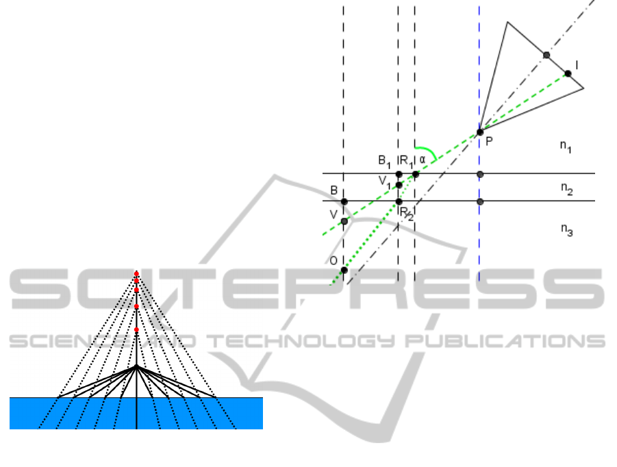
seen in figure 2, the extension of the refracted image
rays (dashed lines) into air leads to several intersec-
tion points, depending on the respective incidence an-
gles and representing multiple virtual viewpoints (red
dots). Because of refraction, there is no collinearity
between the object point in water, the center of pro-
jection of the camera (black dot) and the image point.
On the contrary, all rays following the pinhole cam-
era model intersect in a single point, namely the cen-
ter of projection. This occurrence of multiple virtual
viewpoints in underwater imaging makes it impossi-
ble to infer a single focal length adjustment that can
represent the imaging situation in terms of the pin-
hole camera model correctly. Nevertheless, a relation
between the two imaging situations can be assembled
for the single image rays. It follows the rules of phys-
ical optics and is presented in the following sections.
Figure 2: Multiple viewpoints in underwater imaging.
3.1 Overview
The main idea of our approach is, that the imaging
camera with a constant focal length is working based
on the pinhole camera model. In essence, it does not
know anything about refraction. Hence (see figure 3),
one can assume that the camera is imaging a virtual
object point V, which is situated collinear to the cam-
era’s center of projection P and the image point I. The
real object point O is not situated collinear, as a re-
sult of refraction known from Fermat’s and Snell’s
law. We assume that the camera’s intrinsics and non-
linear distortion terms in air are known. For now, it is
expected that lens distortion is not influenced by re-
fraction and hence can be eliminated by standard in
air distortion correction algorithms in advance. A set
of parameters accounting for refraction is assumed to
be known as well. These comprise the indexes of re-
fraction of the involved media, which are expected to
stay constant. Further known parameters are the per-
pendicular distance from the refractive interface to the
center of projection, the camera’s orientation towards
this interface and the interface thickness.
Stepping back to the assumption of the underwater
camera imaging a virtual object point, we show how
Figure 3: Geometric construction of the location of the vir-
tual object point.
to infer virtual camera parameters following the pin-
hole camera model for the corresponding image ray
using the virtual object point’s location. These vir-
tual parameters belong theoretically to a virtual cam-
era imaging an underwater object point, as if the wa-
ter was eliminated, to the same image point as the real
underwater camera does. The image point in the vir-
tual camera, its center of projection and the real un-
derwater object point are collinear (see figure 4). As
already mentioned before, refraction leads to the per-
ception of an object being closer as it really is and
hence being magnified. This corresponds directly to
the location of the virtual object point. As a conse-
quence, the virtual camera’s focal length differs from
the one of the real camera, because it has to compen-
sate for this magnification. A well known limit case
from physics is a ray with an incidence angle of 90 de-
grees. Only in this case the focal length can simply be
multiplied by the refractive index of water to result in
the corresponding virtual focal length (rule of thumb
for underwater magnification). For incidence angles
differing from this perpendicularity the computation
gets more complicated. The virtual parameters don’t
just comprise focal length but also a new location of
the center of projection and a new orientation to the
refractive interface. The image’s principal point is ex-
pected to stay constant and the skew factor is ignored.
The biggest problem is to find the location of the
virtual object point V. More precisely, if one can find
a rule to locate the virtual object point on the image
ray relative to its real location on the refracted ray (see
figure 3), one can infer the virtual camera parameters
as will be shown. The result is a set of virtual parame-
VISAPP2014-InternationalConferenceonComputerVisionTheoryandApplications
98

ters per image ray. This can lead to a huge number of
parameters, because the number of image rays corre-
sponds to the number of image pixels. These parame-
ters only depend on ray direction which stays constant
from image to image, as long as the camera’s posi-
tion to the refractive interface stays fixed. They are
independent of the imaged scene. Hence, it is possi-
ble to compute all parameters for a single image in a
pre-computation step and reuse them for consecutive
images. The number of parameters can be decreased
if rays with the same properties are summarized. The
only significant properties are the incidence angle to
the refractive interface and the ray’s angle to the opti-
cal axis of the camera.
3.2 Imaging Setup
For our experiments we generate an ideal imaging
setup by using simulated underwater images rendered
with Blender. Simulated images seem to be adequate
for our effort to show the applicability of our theoret-
ical approach for computation of virtual camera pa-
rameters. Advantages are the already known needed
parameters and perfect perspective projection under
the influence of refraction. The imaged scene and
the general camera setup is not restricted. For con-
venience in evaluation we use a simple checker pat-
tern on a plane with known dimensions and location
as imaging target. The plane is located in a way that
most of the image regions are covered by the pattern.
This is especially useful to evaluate our algorithms in
outer image regions, where distortions due to refrac-
tion get severe.
4 VIRTUAL CAMERA
PARAMETERS
4.1 Location of Virtual Object Points
Refraction occurs on the way of the light from the
emitting object point on the transition from water to
glass and from glass to air according to Snell’s law in
a plane through the refractive interface’s normal and
the light ray. The way of the light depends on the dis-
tances it has to pass in the respective media, due to
the fact that light always takes the path for which it
needs the shortest time to travel (Fermat’s law). Most
of the times we do not know where the imaged ob-
ject is located. But we do know the camera’s center
of projection and its orientation to the refractive in-
terface. Hence, when looking along the path of light
from camera direction, we can get an image ray from
pixel coordinates and also know its incidence angle
to the refractive interface. Like can be seen in fig-
ure 3, the virtual object point V lies somewhere on
the extended image ray. We start with the formula for
refraction on a single interface:
n
1
g
+
n
2
b
=
n
2
− n
1
r
(1)
with g being the object distance, b being the image
distance and r being the curvature radius of the inter-
face. For a flat interface system we get r = ∞. After
reorganization we end up with
b = −
n
1
n
2
∗ g. (2)
This is what most physics textbooks teach for the case
of an incidence angle of 90 degree. In this case, there
is no refraction just a magnification. Other incidence
angles are not considered explicitly in most cases.
This formula is used as approximation for small de-
viations from 90 degree. It is obviously independent
of the incidence angle and depends on distances and
the speed of light in the involved media. We assume
that these dependencies do not change if the incidence
angle varies and just a change in direction of the im-
age ray and the refracted ray is happening. When
we consider both media transitions with its refractions
(n
1
= 0) using formula (2), we get
R
1
V =
−
R
1
R
2
n
2
−
R
2
O
n
2
(3)
for the distance from the incidence point R
1
to the vir-
tual object point V on the extended image ray. For a
geometrical representation with an arbitrary but fixed
real object point we have all we need to illustrate the
location of the virtual object point. As can be seen
in figure 3 it is located directly above the real object
point on the perpendicular of the interface. If we vary
the incidence angle or the object position this stays
apparently the same. This statement coincides with
parts of the work of (Bartlett, 1984). The location
of the virtual object point is a controversial topic in
physics. For our purposes we assume that the virtual
object point is always located exactly above the real
object point on the perpendicular of the flat refractive
interface. That this assumption holds is shown in an
experimental way in a later section. Based on this
assumption, one can relate the distances from the in-
terface (perpendicular) to the virtual point and to the
real point incorporating all three involved media by
BV = BO ∗
cosα
p
n
3
2
− sinα
2
+ B
1
R
2
∗
cosα
p
n
2
2
− sinα
2
(4)
like in (Bartlett, 1984) by simple trigonometric rules.
This relationship stays the same for arbitrary loca-
tions of the real object point on the same refracted
ConvertingUnderwaterImagingintoImaginginAir
99
ray, which can be utilized for depth-independent cal-
culations in the following sections.
After revisiting this concept to determine the lo-
cation of the virtual object point, we show how to use
it to infer the virtual camera parameters in the next
subsection.
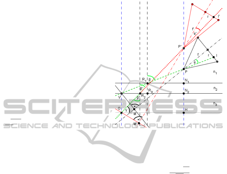
4.2 Parameter Computation
The computation of the virtual camera parameters
is illustrated geometrically in figure 4. As refrac-
tion happens in a plane and following the results of
(Agrawal et al., 2012), the virtual center of projection
P’ lies on the flat interface’s normal through the real
center of projection P (axial camera). The point is de-
termined by the intersection of the rearward extended
refracted ray (green dotted line turning into red) and
that normal. As we know the angle β from the dot
product of the image ray and the interface’s normal
in the camera’s coordinate system as well as the dis-
tances N
1
N
2
corresponding to the interface thickness
and PN
1
corresponding to the perpendicular displace-
ment of the center of projection from the interface, we
can compute nearly all we need for parameter compu-
tation by simple trigonometric rules. Further refrac-
tive angles β
0
and β
00
can be determined by Snell’s law.
Because of perpendicularity, the virtual center of pro-
jection P’ turns to an easy computable distance. Now
the location of the virtual object point V is incorpo-
rated. Since it is located directly above the real object
point and their relationship is depth-independent we
define it to be located exactly on the surface between
water and glass. This fixation makes further simple
trigonometric calculations possible.
As we know the angle α of the image ray to the
optical axis of the camera from image coordinates and
focal length, we know all the angles and distances il-
lustrated in figure 4 except for the virtual focal length
f’ and the virtual camera’s orientation. This orienta-
tion is conditioned by the angle α
0
in an ambiguous
way. For determination of this focal length and ori-
entation we need the rules for magnification of lenses
from physical optics. In figure 4 both, the real (black
triangle) and the virtual camera (red triangle) are il-
lustrated. We want our real object O to appear at the
exact same pixel position on the virtual camera’s im-
age sensor (I’) as is the virtual object point V on the
real camera’s sensor (I). It hast to be in the correct
magnification which is realized by the virtual focal
length and correct positioning of the virtual camera’s
optical axis. The virtual optical axis is determined by
angle α
0
. From α
0
and r the virtual focal length f ’
can be easily calculated. For the calculation of α
0
we
found out that the distances perpendicular to the re-
Figure 4: Geometric construction of the virtual parameters.
spective optical axis (MV and M’O) have to be equal,
so that magnification works properly. Furthermore,
by knowing angle α and the distances VP and OP’
one can calculate α
0
by
α
0
= arcsin
sinα ∗ VP
OP
0
. (5)
In contrast to refraction, which happens in a plane, the
real and the virtual optical axis needs not to be located
in that plane. The virtual optical axis has an ambigu-
ous location, because it is just determined based on an
angle α
0
to the respective ray. Hence, it can be located
on a position anyway around the ray. This is not really
a problem because of the fact that the pixel position
of the ray in the respective image is not altered by
this and the virtual parameters are calculated for this
ray only. An arbitrary but matching virtual orienta-
tion can be computed with angle α
0
and the definition
of the dot product as the angle between two vectors.
One being the refracted ray and the other being the
optical axis with two degrees of freedom. Based on
the vector of the optical axis both missing coordinate
axes can be computed in a similar way.
These virtual parameters essentially convert un-
derwater imaging into imaging in air. If the camera
is oriented perpendicular it leads to some simplifica-
tions during computation.
VISAPP2014-InternationalConferenceonComputerVisionTheoryandApplications
100
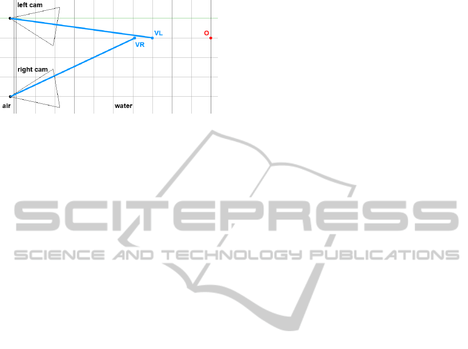
Figure 5: Stereo setup with different virtual object points.
5 3D-RECONSTRUCTION
In this experiment we use the concept for the relation
between the location of virtual object points and real
object points in a stereo 3D reconstruction problem.
This should underline the applicability of this con-
cept. Furthermore, the results are compared with the
results of a stereo 3D reconstruction based on a naive
in-situ stereo camera calibration ignoring refraction.
A stereo camera system is generated with Blender
as can be seen in figure 5. The cameras are located
40 cm apart in a horizontal converging formation of
10 degree per camera. The perpendicular distance to
the flat refractive interface with a thickness of 1cm
amounts to 2cm for each camera. The refractive in-
dexes are respectively 1 for air, 1.6 for glass and 1.33
for water. The focal length of both cameras is 27mm,
with an image resolution of 1920x1080, square pix-
els and a horizontal sensor size of 22.3mm. Hence,
all needed parameters are known in advance (corre-
sponding to camera calibration in air) and radial im-
age distortion can be set to zero. Both cameras image
a plane with a checker pattern at a certain distance.
The checker corners on that plane are used as feature
points and their respective 3D locations are known.
We tried to cover as much of the overlapping image
region with the pattern. For each corresponding fea-
ture pair the respective image ray is calculated in a
left-handed world coordinate frame with its origin on
the foot of perpendicular of the left camera on the
water-sided interface. The z-axis is pointing into the
water, the y-axis points upward and the x-axis to the
left. The two rays are emitted from a different virtual
object point (VL and VR). However, both rays corre-
spond to the same real object point O. The two virtual
object points are not likely to intersect in the same z-
value as long as their respective rays have different
incident angles. What we are able to do is to com-
pute the intersection of just the x- and y-values of both
rays. The results are differing in their z-values as can
be seen exemplary in figure 5. Now we use formula
(4) to compute the z-value of the real object point.
The two new z-values should be nearly the same and
we take their mean as object depth. The x- and y-
values stay the same. With this easy method we have
inferred the 3D coordinates of our object from just a
virtual object point and refraction is handled physi-
cally plausible.
6 RESULTS
The results of our computation of virtual camera pa-
rameters are tested in an experimental way. The
rendering sequence to check if our computed virtual
camera parameters match the situation works as fol-
lows. We render an underwater image of our target
with Blender with known parameters. We compute
the virtual parameters for one feature point. After-
ward, we use these parameters in Blender to render
a new image of our target, but this times in air. The
result should be an image with the feature point at ex-
actly the same image location and in the same mag-
nification as in the underwater image. This feature
point is now the result of a perspective projection and
refraction is eliminated for this particular image pixel.
The camera is imaging a plane with a checker pattern
in an underwater environment. The refractive indexes
are respectively 1 for air, 1.6 for glass and 1.33 for
water. The interface has a thickness of 1cm and the
camera is placed 2cm in perpendicular direction away
from it with a horizontal angle of 10 degree. Its fo-
cal length is 27mm. This matches the left camera in
figure 5. Because of the required exact placement and
configuration of the virtual camera, this can not be
evaluated in the desired accuracy with real image se-
tups in a reasonable way.
One rendered result can be seen in figure 6. The
corresponding feature points are marked with a cir-
cle. Manual visual evaluation results in a difference
of zero pixel between both feature points. The green
lines are drawn supplementary to illustrate the distor-
tions in the underwater image and the truly straight
chessboard lines in the in air image. Because of the
already mentioned ambiguous orientation of the vir-
tual camera, the in air rendered image is rotated. The
pixel position is not affected by this as can bee seen
and as was explained before. The virtual focal length
for this case is 36.632mm, the virtual center of pro-
jection is at a distance of 2.608cm from the refractive
interface and the camera’s rotation matrix amounts to
R =
0.9718 0.2121 0.1027
−0.0909 −0.0644 0.9938
0.2174 −0.9751 0.0433
.
Further tests on several random feature points re-
ConvertingUnderwaterImagingintoImaginginAir
101
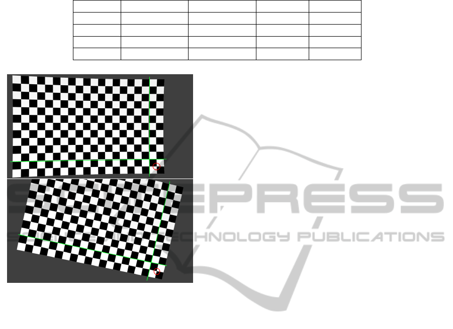
Table 1: 3D reconstruction errors
IN-SITU(1m) IN-SITU(2m) OUR(1m) OUR(2m)
3D Error 6.831cm 13.559cm 0.32cm 1.074cm
x-Error 6.571cm 12.92cm 0.08cm 0.15cm
y-Error 0.076cm 0.152cm 0.035cm 0.077cm
z-Error 1.714cm 3.65cm 0.285cm 1.042cm
Figure 6: Comparison of the rendered underwater image
(top) and the inferred in air rendering (bottom) with the cor-
responding ray (image pixel) marked by the red circle.
sulted in a mean deviation of at most 1 pixel. This
shows that our method is well applicable for our sce-
nario.
For stereo 3D reconstruction we used 204 feature
points on a plane at a distance of 1m and 228 fea-
ture points on a plane at a distance of 2m from the
refractive interface. The planes are parallel to the in-
terface and all 3D locations of the feature points are
known in advance. The results of our method and the
results of a stereo 3D reconstruction based on a naive
in-situ stereo camera calibration ignoring refraction
are compared in table 1. The denoted errors are the
3D mean euclidean distance as well as the euclidean
distances per coordinate direction between measured
and real 3D points. Our results are significantly better
than those of the in-situ method. The huge error in x-
direction of the in-situ method amounts from false rel-
ative orientation parameters from in-situ stereo cam-
era calibration. The ignored magnification by refrac-
tion leads to a shift of the camera behind its real po-
sition and to a smaller angle in the converging cam-
era setup. This false camera configuration somehow
compensates the triangulation error in z-direction at
the cost of a shift in x-direction leading to an overall
severe error in 3D location. On the contrary, our val-
ues match the 3D locations at this comparatively large
imaging distances pretty well in all dimensions.
7 CONCLUSIONS
We presented a new method to convert an underwater
image to imaging conditions in air with the aid of a
set of virtual camera parameters for each image ray.
Rays with the same properties can be summarized.
Our method is based on rules of physical optics. The
virtual parameters can be computed for one image in
a pre-processing step. They can be reused for every
consecutive image from that camera. With known vir-
tual parameters, computer vision algorithms relying
on the pinhole camera model can now be executed
for the underwater images. In an experimental way,
we show that our method matches our imaging condi-
tions. Our results are tested on simulated image data
allowing for ground truth comparison. This proce-
dure shows that our theoretical results are correct and
applicable. Our underwater imaging model makes it
possible to infer parameters of an underwater camera
from its calibration in air. Hence, we avoid a cumber-
some and expensive in-situ calibration.
In a further experiment we show that our used
concepts can be incorporated into stereo 3D recon-
struction. The results are significantly better than the
results of a naive in-situ stereo calibration with fol-
lowing triangulation. This experiment underlines the
applicability of our method for underwater imaging.
Further validation on real image data and a compar-
ison with naive in-situ, as well as with more mature
calibration approaches is needed and is part of our fu-
ture work.
REFERENCES
Agrawal, A., Ramalingam, S., Taguchi, Y., and Chari, V.
(2012). A theory of multi-layer flat refractive geom-
etry. In 2012 IEEE Conference on Computer Vision
and Pattern Recognition (CVPR), pages 3346 – 3353.
Bartlett, A. A. (1984). Note on a common virtual image.
American Journal of Physics, 52(7):640 – 643.
Beall, C., Lawrence, B. J., Ila, V., and Dellaert, F.
(2010). 3D reconstruction of underwater structures.
VISAPP2014-InternationalConferenceonComputerVisionTheoryandApplications
102

In 2010 IEEE/RSJ International Conference on Intel-
ligent Robots and Systems (IROS), pages 4418 – 4423.
Brandou, V., Allais, A. G., Perrier, M., Malis, E., Rives,
P., Sarrazin, J., and Sarradin, P. M. (2007). 3D re-
construction of natural underwater scenes using the
stereovision system IRIS. In OCEANS 2007 - Europe,
pages 1–6.
Chang, Y.-J. and Chen, T. (2011). Multi-view 3D recon-
struction for scenes under the refractive plane with
known vertical direction. In ICCV’11, pages 351 –
358.
Chari, V. and Sturm, P. (2009). Multiple-view geometry of
the refractive plane. In Proceedings of the 20th British
Machine Vision Conference, London, UK.
Eustice, R. M., Pizarro, O., and Singh, H. (2008). Visu-
ally augmented navigation for autonomous underwa-
ter vehicles. IEEE Journal of Oceanic Engineering,
33(2):103–122.
Ferreira, R., Costeira, J. P., and Santos, J. A. (2005). Stereo
reconstruction of a submerged scene. In Proceedings
of the Second Iberian conference on Pattern Recogni-
tion and Image Analysis - Volume Part I, IbPRIA’05,
pages 102–109.
Gedge, J., Gong, M., and Yang, Y. (2011). Refractive epipo-
lar geometry for underwater stereo matching. In 2011
Canadian Conference on Computer and Robot Vision
(CRV), pages 146–152.
Gracias, N. and Santos-Victor, J. (2000). Underwater video
mosaics as visual navigation maps. Computer Vision
and Image Understanding, 79:66 –91.
Ishibashi, S. (2011). The study of the underwater camera
model. In OCEANS, 2011 IEEE - Spain, pages 1–6.
Johnson-Roberson, M., Pizarro, O., Williams, S. B., and
Mahon, I. (2010). Generation and visualization
of large-scale three-dimensional reconstructions from
underwater robotic surveys. Journal of Field Robotics,
27(1):21–51.
Jordt-Sedlazeck, A. and Koch, R. (2012). Refractive cali-
bration of underwater cameras. In Proceedings of the
12th European conference on Computer Vision - Vol-
ume Part V, ECCV’12, pages 846–859.
Ke, X., Sutton, M. A., Lessner, S. M., and Yost, M. (2008).
Robust stereo vision and calibration methodology for
accurate three-dimensional digital image correlation
measurements on submerged objects. Journal of
Strain Analysis for Engineering Design, 43(8):689–
704.
Kunz, C. and Singh, H. (2008). Hemispherical refrac-
tion and camera calibration in underwater vision. In
OCEANS 2008, pages 1–7.
Kunz, C. and Singh, H. (2010). Stereo self-calibration for
seafloor mapping using AUVs. In Autonomous Under-
water Vehicles (AUV), 2010 IEEE/OES, pages 1–7.
Kwon, Y.-H. and Casebolt, J. B. (2006). Effects of light
refraction on the accuracy of camera calibration and
reconstruction in underwater motion analysis. Sports
Biomechanics / International Society of Biomechanics
in Sports, 5(2):315–340.
Lavest, J. M., Rives, G., and Lapreste, J. T. (2003). Dry
camera calibration for underwater applications. Mach.
Vision Appl., 13(5-6):245 – 253.
Li, R., Li, H., Zou, W., Smith, R. G., and Curran, T. A.
(1997). Quantitative photogrammetric analysis of
digital underwater video imagery. IEEE Journal of
Oceanic Engineering, 22(2):364–375.
Maas, H.-G. (1995). New developments in multimedia
photogrammetry. Symposium A Quarterly Journal In
Modern Foreign Literatures, 8(3):150 – 5.
McKinnon, D., He, H., Upcroft, B., and Smith, R. N.
(2011). Towards automated and in-situ, near-real time
3-d reconstruction of coral reef environments. In
OCEANS’11 MTS/IEEE Kona Conference.
Meline, A., Triboulet, J., and Jouvencel, B. (2010). A cam-
corder for 3D underwater reconstruction of archeolog-
ical objects. In OCEANS 2010, pages 1–9.
Pessel, N., Opderbecke, J., and Aldon, M. J. (2003). An ex-
perimental study of a robust self-calibration method
for a single camera. In Proceedings of the 3rd Inter-
national Symposium on Image and Signal Processing
and Analysis, 2003. ISPA 2003, volume 1, pages 522–
527.
Pizarro, O., Eustice, R. M., and Singh, H. (2009). Large
area 3-D reconstructions from underwater optical
surveys. IEEE Journal of Oceanic Engineering,
34(2):150–169.
Sedlazeck, A. and Koch, R. (2011). Calibration of hous-
ing parameters for underwater Stereo-Camera rigs. In
Proceedings of the British Machine Vision Confer-
ence, pages 118.1 – 118.11.
Sedlazeck, A. and Koch, R. (2012). Perspective and non-
perspective camera models in underwater imaging -
overview and error analysis. In Outdoor and Large-
Scale Real-World Scene Analysis, volume 7474 of
Lecture Notes in Computer Science. Springer Berlin
Heidelberg.
Sedlazeck, A., Koser, K., and Koch, R. (2009). 3D recon-
struction based on underwater video from ROV kiel
6000 considering underwater imaging conditions. In
OCEANS 2009 - EUROPE, pages 1–10.
Shortis, M., Harvey, E., and Abdo, D. (2009). A review
of underwater stereo-image measurement for marine
biology and ecology applications. In Oceanography
and Marine Biology, volume 20092725, pages 257–
292. CRC Press.
Shortis, M. R. and Harvey, E. S. (1998). Design and cali-
bration of an underwater stereo-video system for the
monitoring of marine fauna populations. Interna-
tional Archives Photogrammetry and Remote Sensing,
32(5):792–799.
Silvatti, A. P., Salve Dias, F. A., Cerveri, P., and Barros,
R. M. (2012). Comparison of different camera calibra-
tion approaches for underwater applications. Journal
of Biomechanics, 45(6):1112–1116.
Telem, G. and Filin, S. (2010). Photogrammetric modeling
of underwater environments. ISPRS Journal of Pho-
togrammetry and Remote Sensing, 65(5):433–444.
Treibitz, T., Schechner, Y., Kunz, C., and Singh, H. (2012).
Flat refractive geometry. IEEE Transactions on Pat-
tern Analysis and Machine Intelligence, 34:51–65.
Yamashita, A., Kato, S., and Kaneko, T. (2006). Robust
sensing against bubble noises in aquatic environments
with a stereo vision system. In Proceedings 2006
IEEE International Conference on Robotics and Au-
tomation, 2006. ICRA 2006, pages 928–933.
ConvertingUnderwaterImagingintoImaginginAir
103
