
Visualization of Varying Hierarchies by
Stable Layout of Voronoi Treemaps
Sebastian Hahn
1
, Jonas Tr
¨
umper
1
, Dominik Moritz
2
and J
¨
urgen D
¨
ollner
1
Hasso-Plattner-Institute, Potsdam, Germany
Keywords:
Hierarchical Visualization, Voronoi Treemaps, Stable Layout, Changing Hierarchies.
Abstract:
Space-restricted techniques for visualizing hierarchies generally achieve high scalability and readability (e.g.,
tree maps, bundle views, sunburst). However, the visualization layout directly depends on the hierarchy, that
is, small changes to the hierarchy can cause wide-ranging changes to the layout. For this reason, it is difficult
to use these techniques to compare similar variants of a hierarchy because users are confronted with layouts
that do not expose the expected similarity. Voronoi treemaps appear to be promising candidates to overcome
this limitation. However, existing Voronoi treemap algorithms do not provide deterministic layouts or assume a
fixed hierarchy. In this paper we present an extended layout algorithm for Voronoi treemaps that provides a high
degree of layout similiarity for varying hierarchies, such as software-system hierarchies. The implementation
uses a deterministic initial-distribution approach that reduces the variation in node positioning even if changes
in the underlying hierarchy data occur. Compared to existing layout algorithms, our algorithm achieves lower
error rates with respect to node areas in the case of weighted Voronoi diagrams, which we show in a comparative
study.
1 INTRODUCTION
Space-restricted visualization of hierarchical data has
been a well investigated research field for the last
decades. Although most of the existing techniques per-
form well with respect to scalability, readability, and
the aspect ratio of the items (i.e., the graphical repre-
sentation of hierarchy nodes), the stability of the lay-
out represents a major challenge. If the depiction of
similar hierarchies (e.g., varying hierarchies) does not
expose similar layouts, the usability is substantially re-
stricted. Users need to analyze and correlate the visual-
ization results to compare the hierarchy visualization
and to detect changes.
Guerra-G
´
omez et al. (Guerra-G
´
omez et al., 2013)
define five types of tree-comparison problems. In our
case, we need to discern two comparison problems:
The layout algorithm faces a type 3 problem (“positive
and negative changes in leaf node values with aggre-
gated values in the interior nodes and with changes in
topology”); the user faces a type 1 problem (“positive
and negative changes in leaf node values with aggre-
gated values in the interior nodes [...] and no changes
in topology”). That is, the layout algorithm has to deal
with both topological as well as value changes and
(a) (b)
Figure 1: Chromium Compositor project (approx. 500 files):
Visualization of its hierarchy for two revisions. Despite a
number of changes in 1 month (May 2013) – 314 files
changed, 30 files added, and 18 files deleted – the layout
is stable and we notice significant coherence between the
two images (the nodes’ unique ids are mapped to color).
shall produce a layout that exhibits only few topologi-
cal changes but still represents value changes.
In other words, we refer to such a layout algo-
rithm’s ‘tolerance’ against changes in varying input
hierarchy-data with respect to the arrangement and
layout of resulting visual representations as layout
stability. Layout stability is considered essential for
effectively and efficiently performing visual analysis
tasks such as comparing hierarchies and attributes of
such hierarchies’ nodes, and tracking changes to hi-
50
Hahn S., Trümper J., Moritz D. and Döllner J..
Visualization of Varying Hierarchies by Stable Layout of Voronoi Treemaps.
DOI: 10.5220/0004686200500058
In Proceedings of the 5th International Conference on Information Visualization Theory and Applications (IVAPP-2014), pages 50-58
ISBN: 978-989-758-005-5
Copyright
c
2014 SCITEPRESS (Science and Technology Publications, Lda.)

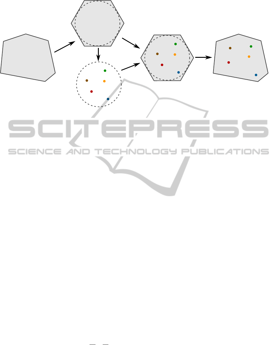
Create Voronoi treemap
Calculate
Power Diagram
AdaptPositionsWeights AdaptWeights
Calculate
Power Diagram
Calculate
Power Diagram
Create random
distribution
Create deterministic
stable distribution
break
Improve distribution
done
a.) b.) c.) d.)
Figure 2: Process of computing a Voronoi treemap with weighted sites.
erarchies over time (Nocaj and Brandes, 2012b; Card
et al., 2006; Hadlak et al., 2010). A key reason for this
fact is that users explore visual representations and
create their own mental maps (Kitchin, 1994). Such
maps significantly aid their orientation in the visual-
ized information space by providing a reference sys-
tem similar to road maps in the physical world. As
with navigation in the physical world, such map is use-
less if changes to the input data result in items not be-
ing placed as expected. Thus, users can only use their
mental map if the context – the spatial position of hier-
archy nodes – is more or less stable, i.e., within some
small frame of placement error. Otherwise, a new men-
tal map has to be constructed. For example, in software
visualization, large sequences of versioned module hi-
erarchies (e.g., source-code trees) demand for a degree
of coherence in corresponding visual representations
to facilitate comprehension of the underlying software
evolution.
Voronoi treemaps appear to be promising candi-
dates to increase layout stability for visualizing vary-
ing hierarchies. Due to the way Voronoi diagrams are
constructed, changes in the input data (a point distribu-
tion) typically only induce locally constrained changes
to the output. One of the main disadvantages of exist-
ing layout algorithms for Voronoi treemaps (Balzer
et al., 2005; Nocaj and Brandes, 2012a) consists in
using a random initial distribution, which can result
in essentially different depictions of similar hierar-
chies. We present an approach for deterministically
computing an initial point distribution as input for the
Voronoi Treemap computation stage instead of the ran-
dom initial distribution used by Nocaj and Brandes
(see Fig. 2a). As the distribution algorithm is toler-
ant against changes in the input hierarchy, we ensure
that hierarchy nodes are position-stable in the result-
ing layout, and achieve a high degree of layout sta-
bility for varying hierarchies. Further, our approach
reduces the error of achieved target areas for weighted
Voronoi treemaps. For it, we show three optimizations
to the latest algorithm: (see Fig. 2b) a less restrictive
but holding criteria for the prevention of empty cells,
(see Fig. 2c) a different calculation for increasing and
decreasing the cell sizes through the iterative process,
and (see Fig. 2d) a more precise break condition. We
show an application of our Voronoi treemap layout
algorithm in the field of software visualization, exem-
plified for the case of a sub-module of the open-source
web browser Chromium
1
, the Chromium Compositor
(cc) project (as shown in Fig. 1).
This paper is structured as follows. Section 2 gives
a brief overview about related and previous work on
layout stability, mental maps and treemaps, as well as
techniques used for shape transformations. A theoret-
ical model for varying hierarchical data is given in
Section 3. Section 4 describes the workflow and pro-
posed algorithms to render Voronoi treemaps layout
stable with respect to varying hierarchical data. In Sec-
tion 5 our improvements to the latest Voronoi treemap
algorithm by Nocaj and Brandes (Nocaj and Brandes,
2012a) are shown to reduce the number of iterations
and to increase precision of target-area sizes. The eval-
uation of our improvements to the Algorithm of Nocaj
and Brandes is presented in Section 6. Finally, Sec-
tion 7 concludes this paper and gives an outlook on
possible future work.
2 RELATED WORK
Since the invention of Treemaps by Johnson and
Shneiderman (Johnson and Shneiderman, 1991),
space-restricted hierarchical visualization has been im-
proved along the dimensions of item ordering, aspect-
ratio, readability, and stability. While the original
Slice’n dice treemap layout (Shneiderman, 1992) cre-
ates representations with good stability, its items can
have imbalanced aspect ratios that aggravate overall
readability and size comparison between items. Other
layout techniques such as Squarified (Bruls et al.,
2000) or Strip (Shneiderman and Wattenberg, 2001)
focus on creating items with an aspect-ratio close to
one, but are less layout stable (Sud et al., 2010).
1
http://www.chromium.org, last accessed 07/25/2013
VisualizationofVaryingHierarchiesbyStableLayoutofVoronoiTreemaps
51

As outlined above, for our visual-analysis tasks,
in particular the recognition of a hierarchies’ nodes,
the memorability of item positions is a primary goal.
The InfoSky, presented by Andrews et al., uses a force-
based node placement and additively weighted power
diagrams for the visualization of hierarchically struc-
tured documents (Andrews et al., 2002). Kuhn et al.
present a non-space-restricted approach that creates
a so-called software landscape or software map by
applying a mountain metaphor to create a consistent
visualization (Kuhn et al., 2008). For it, a multidimen-
sional scaling (MDS) algorithm creates a distribution
of the hierarchy nodes in visual space. Afterwards, a
hill shading based on the lines of code of each artifact
is applied. This use of MDS leads to a high degree
of consistency over several variants of a hierarchy but
does not allow for visualizing the hierarchy’s structure.
To achieve higher layout stability, Tak and Cockburn
present a rectangular-based treemap layout-algorithm –
Hilbert and Moore treemaps (Tak and Cockburn, 2013)
– that uses the space-filling property of Hilbert and
Moore curves. By this, the approach prevents spa-
tial discontinuity with respect to the items’ siblings.
Reusing an initial reference layout for subsequent lay-
out computations based on Voronoi treemaps (Nocaj
and Brandes, 2012b) also partially addresses this is-
sue. It assumes, though, as input a single version of the
same hierarchy (or sub-hierarchies thereof). Whenever
this hierarchy changes, the reference layout becomes
invalid and thereby unusable. To achieve layout sta-
bility in Voronoi treemaps, the use of deterministic
algorithms for computing an initial point distribution
instead of random ones is essential. Due to the fact that
Voronoi treemaps can be used with arbitrary convex
root polygons, generalizable polygon coordinates are
needed. A common way to achieve this is the use of
generalized barycentric polygon coordinates, or Wach-
spress coordinates (Wachspress, 1975). These coordi-
nates, which are well defined for convex polygons, al-
low the description of a point inside the polygon with
respect to a polygon’s vertices. Floater et al. further
present an algorithm using Wachspress coordinates to
transform the coordinates of points from inside an ini-
tial polygon into a target polygon (Floater et al., 2006).
Our goal combines the above challenges: We want
to create a visualization that allows for implicitly
identifying unchanged and changed hierarchy nodes
across multiple variants of a hierarchical dataset. That
is, the stability property of our computed layout shall
enable users to distinguish (un)changed nodes by their
relatively (un)stable spatial position and, thereby, also
the recognizability of structural patterns (groups of un-
changed hierarchy nodes). By this, they are effectively
able to identify trends in the visualization of those
data, to compare depictions of different states.
3 VARYING HIERARCHICAL
DATASETS
There exists a wide range of varying hierarchical
datasets. To illustrate this diversity, we pick two exam-
ples, illustrating a set of change operations that induce
the variation of the datasets, before we define a formal
model of the datasets that we consider in this paper.
File-Systems on Hard disks
Files on a hard
disk are structured strongly hierarchical (excluding
links) using folders. In addition to this parent-child-
relationship meta information on files, e.g., the at-
tributes size and modification date, exist. A folder’s
size is then the aggregation of the sizes of all files con-
tained in such folder. Furthermore, a file system can
be modified by editing files, and through it modify-
ing their file size (operation changeAttribute), deleting
files as well as folders, and adding new files or folders.
Tree of Life
The tree of life shows a hierarchi-
cal structure of different organisms (the tree’s leafs)
grouped by species. As in the file-system example, at-
tributes exist for the leafs. A typical attribute here is
an organism’s population. Analogous to the file sys-
tem, these attributes change over time, too (changeAt-
tribute). Organism or even species become extinct
(delete) while others evolve (add).
A Formal Model
We define a formal model for vary-
ing hierarchical dataset
H = (N, E)
, which contains a
set of nodes
N = {n
0
, ..., n
i
}
and a set of versioned
edges E = {E
0
, ..., E
j
} as follows:
E = {k
0
, ..., k
l
} k = (n
p
, n
c
) (1)
k
in
E
are considered as edges between nodes de-
scribed by a tuple of nodes (a parent
n
p
and a child
node
n
c
) with the following properties: (a) Only one
tuple exists in E where
n
p
= null
and through this the
child of that
n
p
is considered as root node. (b) Every
child node has only one unique parent node. (c) There
are no (transitive) cycles in E.
Hence, a tuple
T = (N, E
i
∈E)
defines one variant
of our hierarchical dataset. We say that subsequent
variants of such tuples are similar to each other, i.e.,
∀
i∈[0, j−1]
: T
j
∼T
j+1
. We further define a function
uid :
IVAPP2014-InternationalConferenceonInformationVisualizationTheoryandApplications
52

N ×E → N
that yields a unique identifier per path
p : N ×E → N ×... ×N such that:
∀
n
i
,n
j
∈N,E∈E
: p(n
i
, E) 6= p(n
j
, E) ⇔ (2)
uid(n
i
, E) 6= uid(n
j
, E)
Here,
p(n, E)
returns the path from node
n
to the
root node
n
r
defined by
E
. Note that each variant
E ∈
E
can define a different path
p
for a node
n ∈ N
. In
other words, our data model considers nodes that are
moved in
H
as different nodes and they will have more
than one unique identifier
uid
. Last, there exists a set
of functions
attr
i
: N ×E → R
returning numerical
attributes per node n ∈ N and versioned edges E.
4 A STABLE INITIAL
DISTRIBUTION
Nocaj and Brandes construction of Voronoi cells is de-
terministic – except that they start with nondetermin-
istic initial positions for the Voronoi sites. To achieve
stability, we thus need to find a method that is able
to create deterministic initial positions. That is, our
approach has to fulfill the following requirements:
•
The initial-distribution algorithm for the Voronoi
sites has to be deterministic.
•
If change operations such as add or delete occur
to a parent node, they should not affect positions
of its children already positioned in an earlier evo-
lution step.
•
The placement of sites relative to each other has to
be stable, even if polygon’s shape of their parent
has changed.
•
changeAttribute operations on nodes should only
cause small changes in the resulting layout.
Voronoi treemaps allow for using arbitrary convex
polygons as root item, within which any subsequent
direct and indirect child items are contained. For each
created shape that represents a child node, the algo-
rithm can further be applied recursively to this node’s
children.
We start with a target polygon having a given num-
ber of vertices (corners
c
) that represent the root item
in which a set of Voronoi sites
(S)
should be dis-
tributed. Next, we calculate a regular polygon with the
same number of vertices (Fig. 3a). Given a set of nodes
(S)
, which are assumed to have a uniquely identifier,
we are able to define consistent Cartesian coordinates
in a unit square for each node. In our case, we compute
such unique identifier (
uid
) as a hash
<< x, y >>
(an
integer) from a node’s path
p
. We then encode the first
and last half of this hash with
x ∈[0..1]
and
y ∈ [0..1]
.
Next, these two coordinates are transformed into the
incircle of the regular polygon (Fig. 3b and 3c) by cal-
culating polar coordinates (see Equations in (3)).
c = numberOfPolygonVertices
apothem = cos
π
c
<<x, y>> = hash
x
0
y
0
=
x
y
−
0.5
0.5
r = apothem ·
p
x
02
+ y
02
φ = ±arccos
x
0
r
(3)
As a last step, we compute Wachspress coordinates
(Wachspress, 1975) for the regular polygon and the
sites distributed within. They then describe the sites
position inside a convex polygon as weighted terms of
the polygon’s vertices. By using the vertices’ weights,
each point of the distributed sites is transformed into
the target polygon (Fig. 3d) (Floater et al., 2006).
Since it is guaranteed both that the target polygons in
Voronoi treemaps are convex at any time, and that the
incircle and Wachspress coordinates are well defined
for convex polygons, the whole workflow effectively
ensures that the distributed points are always placed
inside the respective target polygon.
As an additional benefit, we do not need to recom-
pute the Wachspress coordinates’ weights of a poly-
gon if the target polygon’s vertices change their po-
sition slightly while polygons number of vertices re-
mains constant. This can happen, e.g., when changes
in the item’s occur. It thereby allows for a fast recalcu-
lation of the target distribution. The Wachspress coor-
dinates only need to be recomputed if the number of
vertices of the target polygon increase or decrease.
5 OPTIMIZED LAYOUT
COMPUTATION
After the initial distribution, the actual Voronoi
treemap is computed (Fig. 2 b,c,d). Although the orig-
inal algorithm (Nocaj and Brandes, 2012a) describes
a rather fast way for computing Voronoi treemaps, we
identified several optimizations for achieving more
precise results with respect to the size of target area
size of created Voronoi cells. These optimizations con-
cern the functions used in the iterative positioning
process (Fig. 2 b,c) as well as the break condition
(Fig. 2 d) that decides weather a distribution is suf-
ficiently precise.
VisualizationofVaryingHierarchiesbyStableLayoutofVoronoiTreemaps
53
c=6
c=6
(a)
(c)
(d)
(b)
Regular
Target
Polygon
Polygon
Incircle
Figure 3: Workflow for computing a deterministic initial site distribution within a target polygon (left). (a) A regular polygon
with the same number of vertices as the target polygon is created. (b) Sites are distributed by our deterministic approach into a
unit circle and (c) transformed into the incircle of a regular polygon. (d) The regular polygon and the sites distributed within
are transformed into the target polygon by using Wachspress coordinates.
5.1 Precision of Target-Area Size
As the initial positioning of the Voronoi sites does
not necessarily reflect the targeted weights, Nocaj and
Brandes propose an iterative optimization based on
Lloyd’s algorithm. Lloyd’s algorithm, also known as
Voronoi relaxation, in its original form is used to cal-
culate Voronoi diagrams where the sites’ location co-
incide with the centroids of its Voronoi cell(Du et al.,
1999).
Nocaj and Brandes use power diagrams to iter-
atively adapt the sites’ weights and positions dur-
ing each iteration. For it, the current areas (current
size of a cell) of the cells are iteratively adapted
towards the target areas (cell size that should be
achieved). That is, they loop through the functions
AdaptPositionsWeights
and
AdaptPositions
un-
til a break condition is satisfied.
As pointed out by Nocaj and Brandes, empty cells
have to be prevented during the iterative optimization
of weights and positions: A centroid is required for
optimizing a site’s position, but cannot be computed
for empty cells. Such a site’s empty cell can emerge if
the site is encircled by a circle defined by the weight of
another site. Consequently, empty cells can be avoided
by limiting the site’s weights such that the constraint
in Equation 4 is satisfied.
∀s,t ∈ S, s 6= t : ||s −t||> max(
√
w
s
,
√
w
t
) (4)
However, Nocaj and Brandes propose a criterion
that is too strong in several cases. They limit the new
site’s weight to the minimum of the distance of the
cell that it belongs to and its maximum weight in Al-
gorithm 1. This often results in many cells being too
small and thus – counterintuitively – especially cells
that should be very small are far too large.
We propose a weaker limit for a site’s weight as
follows: A site’s weight in
AdaptPositionsWeights
is limited to the minimum distance to any other site,
just like Nocaj and Brandes did in
AdaptWeights
. In
most cases, this criterion is weaker, but it always sat-
isfies the constraint in Equation 4. Our Algorithm 3
uses the same method to determine the distance to the
nearest neighbor as proposed by Nocaj and Brandes
in Algorithm 2. The distances can be calculated by
means of a Voronoi diagram in O(nlog n).
During our experiments, we noticed that the
method of Nocaj and Brandes often results in oscil-
lating site locations, weights, and areas during the iter-
ative optimization. To overcome this problem
f
adapt
is limited to
1 ± ρ
if its first derivative (increas-
ing/decreasing the weight) starts oscillating as de-
scribed in Algorithm 4.
Note that even though the distance is described in Al-
gorithm 3 and 4 as being the distance between two
sites, it can also be computed as twice the distance
to the cell from a site. It is not necessary to know
which site is the nearest neighbor. Also note that most
distances can be calculated as the squared distances
which does not require calculating any square roots.
The effects of our optimizations are shown in
Fig. 4 and are evaluated and discussed in detail in Sec-
tion 6.
IVAPP2014-InternationalConferenceonInformationVisualizationTheoryandApplications
54
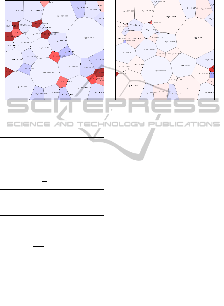
(a) Approach of Nocaj and Brandes (b) Our Approach
Figure 4: Errors in target-area size shown by color (red = too big, white = correct, blue = too small), i.e., color encodes how
much the actual size of a target area deviates from its expected size (given by the respective attribute value mapped to area
size). Comparison between the results from the algorithm of Nocaj and Brandes (left) and our approach (right). In comparison
to Nocaj and Brandes, our optimizations yield higher precision with respect to the error in target-area size .
Algorithm 1: AdaptPositionsWeights
(p, V (S), S,W)
used to adapt the positions and
weights in an iterative optimization algorithm
proposed by Nocaj and Brandes.
1 foreach site s ∈ S do
2 a ← centroid(V
s
)
3 distanceBorder ← min
x∈V
s
||x −s||
4 w
s
← (min(
√
w
s
, distanceBorder))
2
Algorithm 2: AdaptWeights( p, V (S), S,W)
used
to adapt the weights in an iterative optimization algo-
rithm proposed by Nocaj and Brandes.
1 NN ← Nearestneighbor(S)
2 foreach site s ∈ S do
3 A
current
← A(V
s
); // current area
4 A
target
← A(Ω) ·
v(s)
v(p)
; // target area
5 f
adapt
←
A
target
A
current
6 w
new
←
√
w
s
· f
adapt
7 w
max
← ||s −NN
S
||
8 w
s
← (min(w
new
, w
max
))
2
9 w
s
← max(w
s
, ε)
5.2 Break Condition
The iterative optimization to calculate Voronoi dia-
grams where the cells have a target area requires a
break condition (see Fig. 2d) that is satisfied when the
iterative optimization has finished. Nocaj and Brandes
propose to cancel the optimization process when the
sum of area errors is below a certain threshold. They
define the area error as the difference between the cur-
rent area and target area of a Voronoi cell. Furthermore
the maximum number of iterations is limited.
Unfortunately the area error often does not con-
verge to zero and the minimum error that is reached in
a reasonable number of iterations highly depends on
the number of sites and the target areas of the Voronoi
cells. Consequently, the threshold is often reached af-
ter only a few iterations or not reached at all and the
maximum number of iterations is reached. In the first
case more iterations would reduce the sum of area
errors. In the second case fewer iterations would prob-
ably not imply a much higher sum of area errors.
Algorithm 3:
Optimized version of
AdaptPositionsWeights(p, V (S), S,W )
with
less-restrictive empty cell prevention.
1 foreach site s ∈ S do
2 a ← centroid(V
s
)
3 NN ← Nearestneighbor(S)
4 foreach site s ∈ S do
5 w
max
← ||s −NN
S
||
6 w
s
← (min(
√
w
s
, w
max
))
2
VisualizationofVaryingHierarchiesbyStableLayoutofVoronoiTreemaps
55

Algorithm 4:
Optimized version of
AdaptWeights(p, V (S), S,W )
that prevents
“oscillation”.
1 fs ← initialize with zeros
2 NN ← Nearestneighbor(S)
3 foreach site s ∈ S do
4 A
current
← A(V
s
)
5 A
target
← A(Ω) ·
v(s)
v(p)
6 f
adapt
←
A
target
A
current
7 if fs
s
6= 0 and sgn( f
adapt
−1) 6= sgn(fs
s
−1)
then
8 f
adapt
← min(1 + ρ, max( f
adapt
, 1 −ρ))
9 w
new
←
√
w
s
· f
adapt
10 w
max
← ||s −NN
S
||
11 w
s
← (min(w
new
, w
max
))
2
12 w
s
← max(w
s
, ε)
13 fs
s
← f
adapt
We propose a threshold for the difference between
the maximum area error (the maximum error of each
individual cell,
|A
target
s
−A
current
s
|
) of different itera-
tions which could be seen as the slope of the maxi-
mum area error. More formally, the optimization pro-
cess if canceled when
e
diff
< threshold
.
e
diff
is defined
in Equation 5 where
e
−l
is the maximum error
l
itera-
tions ago in a list
L
e
of
l
iterations,
e
b
l
2
c
is the middle
entry of
L
e
and
e
0
is the maximum error in the current
iteration.
e
diff
= max(e
−l
, e
b
l
2
c
) −e
0
(5)
A disadvantage of this method is that the area er-
ror of the resulting Voronoi diagram does not have an
upper bound. However, we know that more iterations
would probably not reduce the area error.
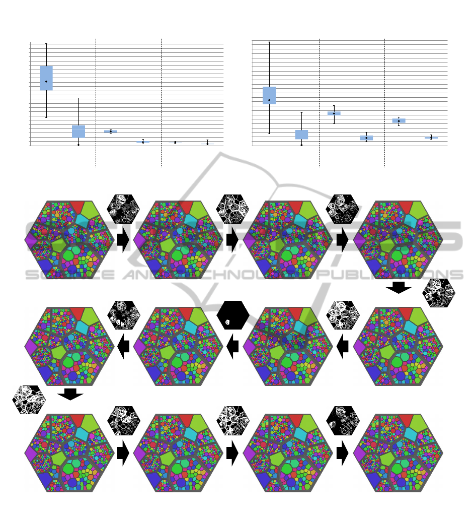
6 COMPARATIVE EVALUATION
To evaluate the optimizations of our approach (
Alg
OA
)
(presented in Section 5) in comparison to the algo-
rithms of Nocaj and Brandes (
Alg
NB
) (Nocaj and
Brandes, 2012a), we tested both algorithms distribut-
ing different numbers of sites within the same parent
polygon. For it, we computed distributions of 10, 50
and 250 sites with random polygon weights with 1000
iterations per distribution. To achieve comparable re-
sults we use the same seed to compute the weights
for each run. The dependent variables of our study are:
Time needed to compute the distribution within 1000
iterations, maximum error of the target sizes and the
sum of target-size errors. Table 1 shows the evaluation
setup with (in)dependent variables in detail.
Table 1: Dependent and independent variables for the com-
parative study (example for 10 sites).
Seed Alg Time Max Err Sum Err
s
1
Alg
OA
t
1
err
max
1
err
sum
1
s
1
Alg
NB
t
2
err
max
2
err
sum
2
s
2
Alg
OA
t
3
err
max
3
err
sum
3
s
2
Alg
NB
t
4
err
max
4
err
sum
4
... ... ... ... ...
s
n
Alg
OA
t
2n−1
err
max
2n−1
err
sum
2n−1
s
n
Alg
NB
t
2n
err
max
2n
err
sum
2n
The mean computation time of
Alg
OA
compared
to
Alg
NB
shows equal results with each number of
sites (Table 2 shows the mean computation times
in detail), our algorithms shows better error rates in
both the maximum area error and the sum of area er-
rors for every number of distributed sites (shown in
Fig. 5 a,b). A paired t-test shows that our method sig-
nificantly decreases both, the maximum area error (10
Sites:
p = 2 ·10
−6
; 50 Sites:
p = 8 ·10
−8
; 250 Sites:
p = 0, 01
) as well as the sum of all area errors (10
Sites:
p = 4 ·10
−4
; 50 Sites:
p = 2 ·10
−6
; 250 Sites:
p = 8 ·10
−8
).
Table 2: Mean computation times for the comparative eval-
uation. The computation times of our algorithm are equal
compared to the ones of Nocaj and Brandes.
Number Of Sites Alg Mean Time
10 Alg
OA
355 ms
10 Alg
NB
353 ms
50 Alg
OA
1686 ms
50 Alg
NB
1701 ms
250 Alg
OA
8937 ms
250 Alg
NB
8914 ms
7 CONCLUSIONS AND
FUTURE WORK
We have presented an extension to an existing layout
algorithm for Voronoi treemaps by using a determin-
istic initial distribution for the Voronoi sites. Since
the resulting layouts are stable with respect to vary-
ing input hierarchies and varying size of items, this
enables the use of Voronoi treemaps for comparing hi-
erarchy variants. Such data sets emerge, e.g., from ver-
sioned source-code trees of software systems. Fig. 6
shows an example of such a varying hierarchy, depict-
ing the cc project from the Chromium Git repository
(branch: master) over several revisions (annotated with
IVAPP2014-InternationalConferenceonInformationVisualizationTheoryandApplications
56
0
0,002
0,004
0,006
0,008
0,01
0,012
0,014
0,016
0,018
0,02
0,022
0,024
0,026
0,028
0,03
0,032
0,034
0,036
0,038
0,04
0,042
0,044
0,046
0,048
Noc+Bran
Our Approach
Noc+Bran
Our Approach
Noc+Bran
Our Approach
Max_ERROR
10 Sites 250 Sites 50 Sites
(a) Maximum target error rates
0
0,01
0,02
0,03
0,04
0,05
0,06
0,07
0,08
0,09
0,1
0,11
0,12
0,13
0,14
0,15
0,16
0,17
0,18
0,19
0,2
0,21
0,22
0,23
0,24
Noc+Bran
Our Approach
Noc+Bran
Our Approach
Noc+Bran
Our Approach
Sum_ERROR
10 Sites 250 Sites 50 Sites
(b) Sum of all node target error rates
Figure 5: Results of the maximum target error rate (a) and the sum of all target error rates (b) evaluated by a comparative study
between (Nocaj and Brandes, 2012a) and our optimization approach to improve the precision of the target areas for different
numbers of sites (10, 50, 250) with randomized weights distributed in their parent node.
Hash: c28df4c Hash: c9f0d06 Hash: d293572 Hash: b38864d
Hash: 045098d Hash: 3d8ab9f Hash: 41512b0 Hash: f826b5f
Hash: a9f0cfd Hash: a4a08d0 Hash: 953e094 Hash: 22898ed
Figure 6: Visualization of the hierarchical folder structure (with about 500 nodes) of 12 revisions from the cc project of the
Chromium Git repository (master). The area of the cells is mapped to the corresponding file size of the represented node.
The nodes’ unique identifier – created from the paths to the root node – is shown as color. For each adjacent layouts, which
represent successive revisions, a difference mask is shown. Unchanged areas are represented by black pixels, while white
pixels indicate differences between the two respective layouts. Although several changes (operations: changeAttribute in 169
files, 5 files added, 2 files deleted) are present in the input data, the resulting layouts are appears as stable and exhibit only few,
local differences. Through it, the layout is memorable over all revisions.
the commit-hashes). Our comparison of target-error
rates further show that we achieve a lower target-error
rate than existing layout algorithms. We conclude that
the resulting layout represents attributes of the input
data more accurately than previous techniques.
As future work, we plan to apply keyframe ani-
mations to blend between the display of the hierarchy
variants. We then plan to evaluate how well users can
track existing hierarchy items in the visualization and
whether the placement of items can be further opti-
VisualizationofVaryingHierarchiesbyStableLayoutofVoronoiTreemaps
57

mized with respect to user expectations. Since com-
puting layouts for large graphs is still too slow for
interactive use, it would likely benefit by porting the
layout algorithm to GPUs. Moreover, we want to add
support for move and rename as possible change oper-
ations.
ACKNOWLEDGEMENTS
The authors would like to thank the anonymous re-
viewers for their valuable comments. This work was
funded by the Research School on ”Service-Oriented
Systems Engineering” of the Hasso-Plattner-Institute
and the Federal Ministry of Education and Research
(BMBF), Germany, within the InnoProfile Transfer re-
search group ”4DnD-Vis” (www.4dndvis.de).
REFERENCES
Andrews, K., Kienreich, W., Sabol, V., Becker, J., Droschl,
G., Kappe, F., Granitzer, M., Auer, P., and Tochtermann,
K. (2002). The infosky visual explorer: exploiting hi-
erarchical structure and document similarities. Infor-
mation Visualization, 1(3-4):166–181.
Balzer, M., Deussen, O., and Lewerentz, C. (2005). Voronoi
treemaps for the visualization of software metrics. In
Proceedings of the 2005 ACM symposium on Software
visualization, pages 165–172. ACM.
Bruls, M., Huizing, K., and Van Wijk, J. J. (2000). Squarified
treemaps. In Data Visualization 2000, pages 33–42.
Springer.
Card, S. K., Sun, B., Pendleton, B. A., Heer, J., and Bodnar,
J. W. (2006). Time tree: Exploring time changing hi-
erarchies. In Visual Analytics Science And Technology,
2006 IEEE Symposium On, pages 3–10. IEEE.
Du, Q., Faber, V., and Gunzburger, M. (1999). Centroidal
voronoi tessellations: Applications and algorithms.
SIAM review, 41(4):637–676.
Floater, M. S., Hormann, K., and K
´
os, G. (2006). A general
construction of barycentric coordinates over convex
polygons. advances in computational mathematics,
24(1-4):311–331.
Guerra-G
´
omez, J. A., Pack, M. L., Plaisant, C., and Shneider-
man, B. (2013). Visualizing Change Over Time Using
Dynamic Hierarchies: TreeVersity2 and the StemView.
IEEE Transactions on Visualization and Computer
Graphics, 19(12):2566–2575.
Hadlak, S., Tominski, C., Schulz, H.-J., and Schumann, H.
(2010). Visualization of attributed hierarchical struc-
tures in a spatiotemporal context. International Jour-
nal of Geographical Information Science, 24(10):1497–
1513.
Johnson, B. and Shneiderman, B. (1991). Tree-maps: A
space-filling approach to the visualization of hierar-
chical information structures. In Visualization, 1991.
Visualization’91, Proceedings., IEEE Conference on,
pages 284–291. IEEE.
Kitchin, R. M. (1994). Cognitive maps: What are they and
why study them? Journal of Environmental Psychol-
ogy, 14(1):1 – 19.
Kuhn, A., Loretan, P., and Nierstrasz, O. (2008). Consistent
layout for thematic software maps. In Reverse Engi-
neering, 2008. WCRE’08. 15th Working Conference
on, pages 209–218. IEEE.
Nocaj, A. and Brandes, U. (2012a). Computing voronoi
treemaps: Faster, simpler, and resolution-independent.
In Computer Graphics Forum, volume 31, pages 855–
864. Wiley Online Library.
Nocaj, A. and Brandes, U. (2012b). Organizing search re-
sults with a reference map. Visualization and Com-
puter Graphics, IEEE Transactions on, 18(12):2546–
2555.
Shneiderman, B. (1992). Tree visualization with tree-maps:
2-d space-filling approach. ACM Transactions on
graphics (TOG), 11(1):92–99.
Shneiderman, B. and Wattenberg, M. (2001). Ordered
treemap layouts. In Proceedings of the IEEE Sym-
posium on Information Visualization 2001, volume
73078.
Sud, A., Fisher, D., and Lee, H.-P. (2010). Fast dynamic
voronoi treemaps. In Voronoi Diagrams in Science and
Engineering (ISVD), 2010 International Symposium
on, pages 85–94. IEEE.
Tak, S. and Cockburn, A. (2013). Enhanced spatial stability
with hilbert and moore treemaps. IEEE Transactions
on Visualization and Computer Graphics, 19(1):141–
148.
Wachspress, E. (1975). A Rational Finite Element Basis.
Academic Press rapid manuscript reproductions. Aca-
demic Press.
IVAPP2014-InternationalConferenceonInformationVisualizationTheoryandApplications
58
