
Fast Segmentation for Texture-based Cartography of whole Slide Images
Gr
´
egory Apou
1
, Beno
ˆ
ıt Naegel
1
, Germain Forestier
2
, Friedrich Feuerhake
3
and C
´
edric Wemmert
1
1
ICube, University of Strasbourg, 300 bvd S
´
ebastien Brant, 67412 Illkirch, France
2
MIPS, University of Haute Alsace, 12 rue des Fr
`
eres Lumiere, 68093 Mulhouse, France
3
Institute for Pathology, Hannover Medical School, Carl-Neuberg-Straße 1, 30625 Hannover, Germany
Keywords:
Whole Slide Images, Biomedical Image Processing, Segmentation, Classification.
Abstract:
In recent years, new optical microscopes have been developed, providing very high spatial resolution images
called Whole Slide Images (WSI). The fast and accurate display of such images for visual analysis by pathol-
ogists and the conventional automated analysis remain challenging, mainly due to the image size (sometimes
billions of pixels) and the need to analyze certain image features at high resolution. To propose a decision
support tool to help the pathologist interpret the information contained by the WSI, we present a new ap-
proach to establish an automatic cartography of WSI in reasonable time. The method is based on an original
segmentation algorithm and on a supervised multiclass classification using a textural characterization of the
regions computed by the segmentation. Application to breast cancer WSI shows promising results in terms of
speed and quality.
1 INTRODUCTION
In recent years, the advent of digital microscopy
deeply modified the way certain diagnostic tasks are
performed. While the initial diagnostic assessment
and the interpretation histopathological staining re-
sults remain a domain of highly qualified experts,
digitization paved the way to semi-automated image
analysis solutions for biomarker quantification and
accuracy control. The emerging use of digital slide
assessment in preclinical and clinical biomarker re-
search indicates that the demand for image analysis
of WSI will be growing. In addition, there is a ris-
ing demand in solutions to integrate multimodal data
sets, e.g. complex immunohistochemistry (IHC) re-
sults with comprehensive genomic, or clinical data.
With the expected increase of the number and quality
of slide scanning devices, along with their great po-
tential for use in clinical routine, increasingly huge
amounts of complex image data (commonly called
Whole Slide Images, WSI) will become available.
Consequently, pathologists are facing the challenge to
integrate complex sets of relevant information, par-
tially based on conventional morphology, and par-
tially on molecular genetics and computer-assisted
readout of single immunohistochemistry (IHC) pa-
rameters (Gurcan et al., 2009).
However, there are still many challenges to the in-
tegration of WSI in routine diagnostic workflows in
the clinical setting (Ghaznavi et al., 2013). Indeed,
these images can contain hundreds of millions or even
billions of pixels, causing practical difficulties for the
storage, transmission, visualization and processing by
conventional algorithms in a reasonable time. The
Fig. 1 presents an example of a WSI of 18000 by
15000 pixels. Moreover, this new technology is still
perceived as ineffective by pathologists who are more
familiar with the use of classical light microscopy.
Current drawbacks that still lead to relatively low ac-
ceptance of this technology include:
• variability in sample preparation (slice thickness,
chemical treatments, presence of air bubbles and
other unexpected elements) and in the acquisition
process (lighting conditions, equipment quality);
• difficulties for human observers to comprehen-
sively analyze quantitative readouts and subtle
variations of intensity, requiring the use of heuris-
tic methods for selecting relevant information,
which introduces a risk of bias (Tavassoli and
Devilee, 2003).
The field of WSI processing also follows the gen-
eral trend in applied sciences of the proliferation of
large databases generated by automated processes.
Increasing quality and performance constraints im-
posed by modern medicine urge for the development
of effective and automatic methods to extract infor-
mation from these databases.
This paper presents a new approach, based on an
object-oriented analysis (segmentation, classification)
309
Apou G., Naegel B., Forestier G., Feuerhake F. and Wemmert C..
Fast Segmentation for Texture-based Cartography of whole Slide Images.
DOI: 10.5220/0004687403090319
In Proceedings of the 9th International Conference on Computer Vision Theory and Applications (VISAPP-2014), pages 309-319
ISBN: 978-989-758-003-1
Copyright
c
2014 SCITEPRESS (Science and Technology Publications, Lda.)
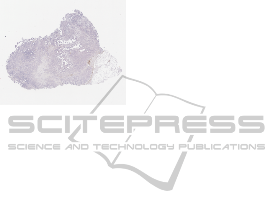
Figure 1: Example of Whole Slide Image.
to establish an automatic cartography of WSI. The
main objective is to propose a decision support tool to
help the pathologist to interpret the information con-
tained by the WSI.
It is widely accepted that segmentation of a full
gigapixel WSI is “impossible” due to time and mem-
ory constraints. We will show that it is in fact possi-
ble to segment such a large image in reasonable time
with minimum memory requirements. Furthermore,
the unexpected potential of simple color histogram to
describe complex textures will be illustrated.
Compared to former works on WSI analysis,
our contributions are: (i) an efficient computational
framework enabling the processing of WSI in reason-
able time, (ii) an efficient texture descriptor based on
an automatic quantification of color histograms and
(iii) a multiclass supervised classification based on
expert annotations allowing a complete cartography
of the WSI.
The paper is organized in 4 sections. First, ex-
isting approaches to analyze WSI are presented (Sec-
tion 2), followed by the different steps of the method
(Section 3). Then, experiments on WSI of breast can-
cer samples are described to evaluate the benefits of
this approach (Section 4). Finally, we conclude and
present some perspectives (Section 5).
2 RELATED WORK
As optical microscopy image analysis is a specific
field of image analysis, a great variety of general tech-
niques to extract or identify regions already exists.
The main distinctive characteristic of the whole slide
images (WSI) is their very large size, which makes
impossible the application of number of conventional
processing, despite of their potential interest.
Signolle and Plancoulaine (Signolle et al., 2008)
use a multi-resolution approach based on the wavelet
theory to identify the different biological components
in the image, according to their texture. The main
limitation of this approach is its speed: about 1 hour to
analyze a sub-image of size 2048 × 2048 pixels, and
several hundred hours for a complete image (60000 ×
40000 pixels).
To overcome this drawback, several methods have
been developed to avoid the need for analyzing entire
images at full resolution. Thus, Huang et al. (Huang
et al., 2010) noted that, to determine the histopatho-
logical grade of invasive ductal breast cancer using a
medical scale called Nottingham Grading System (El-
ston and Ellis, 1991; Tavassoli and Devilee, 2003),
it is important to detect areas of “nuclear pleomor-
phism” (i.e. areas presenting variability in the size
and shapes of cells or their nuclei), but such detection
is not possible at low resolution. So, they propose a
hybrid method based on two steps: (i) the identifica-
tion of regions of interest at low resolution, (ii) multi-
scale resolution algorithm to detect nuclear pleiomor-
phism in the regions of interest identified previously.
In addition, through the use of GPU technology, it is
possible to analyze a WSI in about 10 minutes, which
is comparable to the time for a human pathologist.
Indeed, the same technology is used by Ruiz (Ruiz
et al., 2007) to analyze an entire image (50000 ×
50000) in a few dozen seconds by splitting the im-
age into independent blocks. To manage even larger
images (dozen of gigapixel) and perform more com-
plex analyzes, Sertel (Sertel et al., 2009) uses a clas-
sifier that starts on low-resolution data, and only uses
higher resolutions if the current resolution does not
provide a satisfactory classification. In the same way,
Roullier (Roullier et al., 2011) proposed a multi-
resolution segmentation method based on a model
of the pathologist activity, starting from the coars-
est to the finest resolution: each region of interest
determined at one resolution is partitioned into 2 at
the higher resolution, through a clustering performed
in the color space. This unsupervised classification
can be performed in about 30 minutes (without paral-
lelism) on an image of size 45000 × 30000 pixels.
More recently, Homeyer (Homeyer et al., 2013)
used supervised classification on tile-based multi-
scale texture descriptors to detect necrosis in gi-
gapixel WSI in less than a minute. Their method
shares some traits with our own, but we have a more
straightforward workflow and use simpler texture de-
scriptors on which we will elaborate more later.
The characteristics of our method compared to
former ones are summarized in Table 1.
VISAPP2014-InternationalConferenceonComputerVisionTheoryandApplications
310
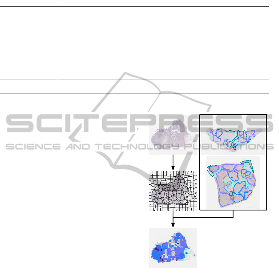
Table 1: Comparison of our method with some existing ones. H&E means Hematoxylin and Eosin, a widely used staining.
Method Pixels Coloration Classes Performance Parallelism
(Ruiz et al., 2007) 10
9
H&E 2 (supervised) 145 s (GeForce 7950 GX2) GPU
(Signolle et al., 2008) 10
9
Hematoxylin,
DAB
5 (supervised) >100 h (Xeon 3 GHz) Unknown
(Sertel et al., 2009) 10
10
H&E 2 (supervised) 8 min (Opteron 2.4 GHz) Cluster of 8
nodes
(Huang et al., 2010) 10
9
H&E 4 (ROI + 3
grades, super-
vised)
10 min (GeForce 9400M) GPU
(Roullier et al., 2011) 10
9
H&E 5 (unsupervised) 30 min (Core 2.4 GHz) Parallelizable
(Homeyer et al., 2013) 10
9
H&E 3 (supervised) <1 min (Core 2 Quad 2.66
GHz)
Unknown
Proposed method 10
8
Hematoxylin,
DAB + PRD
6 (supervised) 10 min (Opteron 2 GHz) Parallelizable
3 METHOD
To achieve a fast and efficient classification of whole
slide images, we propose a methodology enabling to
partition the initial image in relevant regions. This
approach is based on an original segmentation algo-
rithm and on a supervised classification using a textu-
ral characterization of each region.
3.1 Overview
The proposed method relies on two successive steps:
(i) image segmentation into segments or “patches”;
(ii) supervised classification of these segments.
The main challenge of the segmentation step is to
provide a relevant partioning of the image in an effi-
cient way due to the large size of whole slide images.
To cope with this problem, we propose to partition the
image by using a set of horizontal and vertical optimal
paths following image high gradient values.
The classification step is based on a textural ap-
proach where each region is labelled according to its
texture description. This is justified by the fact that,
to produce a decision, a pathologist analyzes the dis-
tribution of objects like cells, and the interaction be-
tween them rather than the objects themselves. We
make the assumption that the distribution of objects
can be described by a textural representation of a re-
gion.
A training set of texture descriptors is computed
from a set of manually annotated images enabling a
supervised classification based on a k-nearest neigh-
bor strategy. The method overview is illustrated in
Fig. 2 and Fig. 3.
Figure 2: Method overview. Left: image under analysis, im-
age partitioning and regions classification. Right: manually
annotated images allowing the construction of the training
set.
3.2 Segmentation
Let f : E → V be a 2D discrete color image defined
over a domain E ⊆ Z
2
with V = [0,255]
3
. Let f
i
de-
notes the scalar image resulting of the projection of f
on its i
th
band. We suppose that E is endowed with
an adjacency relation. A path is a sequence of points
(p
1
, p
2
,... , p
n
) such that, for all i ∈ [1, .. ., n − 1], p
i
and p
i+1
are adjacent points. Let W, H be respec-
tively the width and the height of f . The segmentation
FastSegmentationforTexture-basedCartographyofwholeSlideImages
311
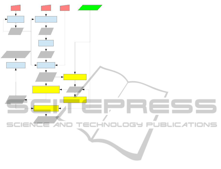
Image
Binary
mask
Patches
Dataset
Classified
patches
Color-coded
map
Annotations
Confusion
matrix
Segmentation
Traversal
Training
Merging
Nearest neighbor
classification
Presentation
Cross-validation
LOD
S Q
Resolution
Description
Described
patches
Figure 3: Data structures and processes. Red boxes rep-
resent parameters, green box represents expert annotations
(ground truth). Blue boxes are image-related operations,
yellow boxes are data mining-related. Gray boxes are data
structures input, exchanged, modified and output by the pro-
cesses.
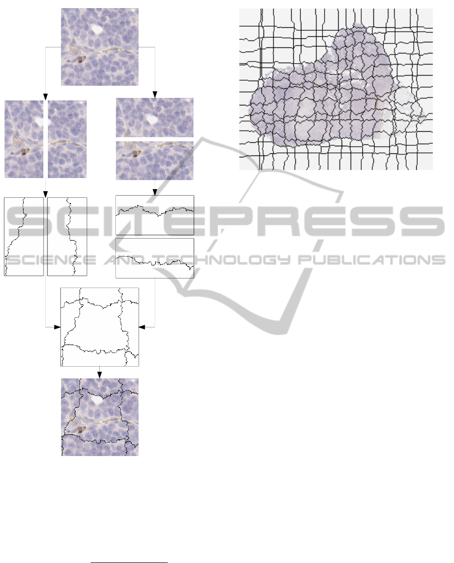
method is based on two successive steps.
First, the image f is partitioned into W /S verti-
cal and H/S horizontal strips, with S > 1 an integer
controlling the width of a strip.
Second, a path of optimal cost is computed from
one extremity of the strip to the other in each image
strip. The cost function is related to the local varia-
tions, hence favoring the optimal path to follow high
variations of the image. More precisely, the local vari-
ation of f in the neighborhood of p is computed as:
g(p) = max
q∈N(p)
d( f (p), f (q)), (1)
where d is a color distance, and N(p) the set of
points adjacent to p. In our experiments we used
d(a,b) = max
i
|a
i
− b
i
| (L
∞
norm) and N(p) = {q |
kp − qk
∞
≤ 1} (8-adjacency).
The global cost associated to a path (p
i
)
i∈[1...n]
of
length n is defined as:
G =
n
∑
i=1
g(p
i
) (2)
From an algorithmic point of view, an optimal
path maximising this summation can be retrieved us-
ing dynamic programming (Montanari, 1971) in lin-
ear time with respect to the number of points in the
strip, hence requiring to scan all image pixels at least
once. To speed up the process, a suboptimal solu-
tion is computed instead by using a greedy algorithm:
starting from an arbitrary seed at an extremity of the
strip, the successive points of the path are added by
choosing, in a local neighborhood, the point q where
g(q) is maximal. By doing so, the values of g are
computed on the fly, only for the pixels neighboring
the resulting path.
Some notable properties of this algorithm are: (i)
its speed due to the fact that not all pixels need to
be processed, (ii) a low memory usage even for large
images because the only required structures are the
current strip and a binary mask to store the result, (iii)
its potential for parallelization, because all strips in a
given direction can be processed independently.
Fig. 4 illustrates the steps of the segmentation
method and Fig. 5 gives an example of the end result.
3.3 Training
To create a training base, the reference images are
segmented into patches. Using the expert annotations,
each patch is associated with a class or label. Then, by
computing a texture descriptor for each patch, we can
create an association between a texture and a group of
labels. A texture can have several labels if it is present
in regions of different classes. As a result, the training
base can be modeled as a function B : T → G where
T is the set of texture descriptors and G = P (L) is the
power set of all labels L.
When |B(t)| 6= 1, the texture t is ambiguous. Sec-
tion 4.2 describes how to measure this phenomenon
and thus quantify the validity of the model. In order
to perform the classification, all B(t) must be single-
tons. To that end, B is updated so that ambiguous
textures are classified as excluded elements.
3.4 Classification
Some authors use distributions of descriptors to de-
scribe textures (Ojala et al., 1996). The chosen de-
scriptors can be arbitrarily complex, and, as a starting
point, we decided to use simple color histograms that
are functions H : V → [0,1] that associate each pixel
color to its frequency in a given patch. Given the fact
that all images were obtained using the same process
and equipment with the same settings, no image pre-
processing was deemed necessary.
In order to perform a supervised multi-class clas-
sification, we opted for a one nearest neighbor clas-
sification because of its simplicity (no assumption
needs to be made on the distribution of the textures
in the descriptor space) and the sufficient amount of
VISAPP2014-InternationalConferenceonComputerVisionTheoryandApplications
312
Horizontal
strips
Horizontal
paths
Vertical
strips
Vertical
paths
Segmentation
mask
Patches
Image
Figure 4: Path computation in horizontal and vertical strips,
leading to an image partition.
training samples available (which turned out to be a
bit excessive with sometimes up to several millions of
elements). For this kind of classification, we measure
the distance between histograms using the euclidean
metric:
d(h
1
,h
2
) =
r
∑
v
(h
2
(v) − h
1
(v))
2
(3)
This choice of descriptor and metric is arbitrary and
will serve as reference for future work.
Figure 5: Example of image partitioning based on our algo-
rithm.
4 EXPERIMENTS AND RESULTS
4.1 Data
Unlike most of the work published on the subject,
our images are obtained using a double-staining pro-
cess (Wemmert et al., 2013). More precisely, we
used formalin-fixed paraffin-embedded breast cancer
samples obtained from Indivumed
R
, Hamburg, Ger-
many. Manual immunohistochemistry staining was
performed for CD8 or CD3/Perforin, and antibody
binding was visualized using 3,3-diaminobenzidine
tetrahydrochloride (DAB, Dako, Hamburg, Germany)
and Permanent Red (PRD, Zytomed, Berlin, Ger-
many). Cell nuclei were counterstained with hema-
toxylin before mounting. As a result, cancerous
(large) and noncancerous (small) cell nuclei appear
blue (hematoxylin), except for lymphocytes which
can be appear red (PRD) and/or brown (DAB) de-
pending on their state.
For our experiments, 7 whole slide images rang-
ing from 1 · 10
8
to 5 · 10
8
pixels have been annotated
by a pathologist using 6 labels: invasive tumor (solid
formations), Fig. 6; invasive tumor (diffusely infiltrat-
ing pre-existing tissues), Fig. 7; intersecting stromal
bands, Fig. 8; DCIS (Ductal Carcinoma In Situ) and
invasive tumor inside ductal structures, Fig. 9; non-
neoplastic glands and ducts, Fig. 10; edges and arti-
facts to be excluded, Fig. 11.
The annotations do not explicitly provide quantifi-
able cell characteristics that could be used to design
a medically relevant cell-based region identification.
Instead, they take the form of outlines that may or
may not match visual features (Fig. 12). Even though
some of these seem obvious, like the background, it is
FastSegmentationforTexture-basedCartographyofwholeSlideImages
313
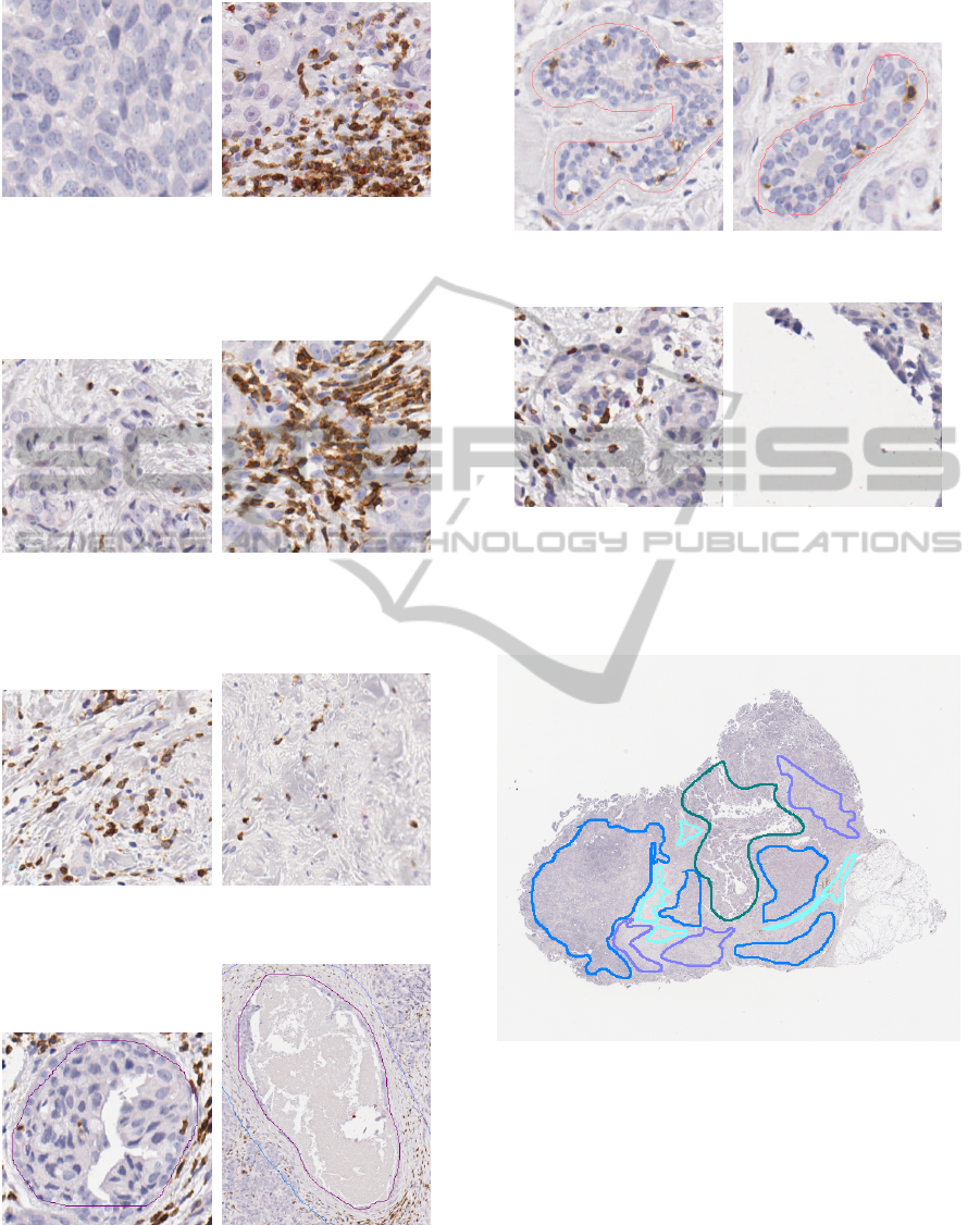
Figure 6: Annotation: Invasive tumor (solid formations).
Description: High concentration of cancerous cells.
Note: All classes can contain foreign objects as can be seen
on the right, and sometimes the same objects (foreign or
not) can be seen in several classes (compare with Fig. 7).
Figure 7: Annotation: Invasive tumor (diffusely infiltrating
pre-existing tissues).
Description: Cancerous cells disseminated in noncancerous
tissue.
Figure 8: Annotation: Intersecting stromal bands.
Description: Connective tissue.
Figure 9: Annotation: DCIS and invasion inside ductal
structures.
Description: A Ductal Carcinoma In Situ refers to cancer
cells within the milk ducts of the breast.
Figure 10: Annotation: Nonneoplastic glands and duct.
Description: Noncancerous structures.
Figure 11: Annotation: Edges and artefacts to be excluded.
Description: Nonbiological features (background,
smudges, bubbles, blurry regions, technician’s hair, ...) and
damaged biological features (borders, defective coloration,
missing parts, ...).
Figure 12: Expert annotations; the regions are outlined,
each color represents a class; excluded regions (dark green)
are given as examples, which is why the image is not fully
annotated.
not easy for an untrained eye to establish a set of in-
tuitive rules that would explain the expert’s opinion,
even after trying some simple visual filters (quanti-
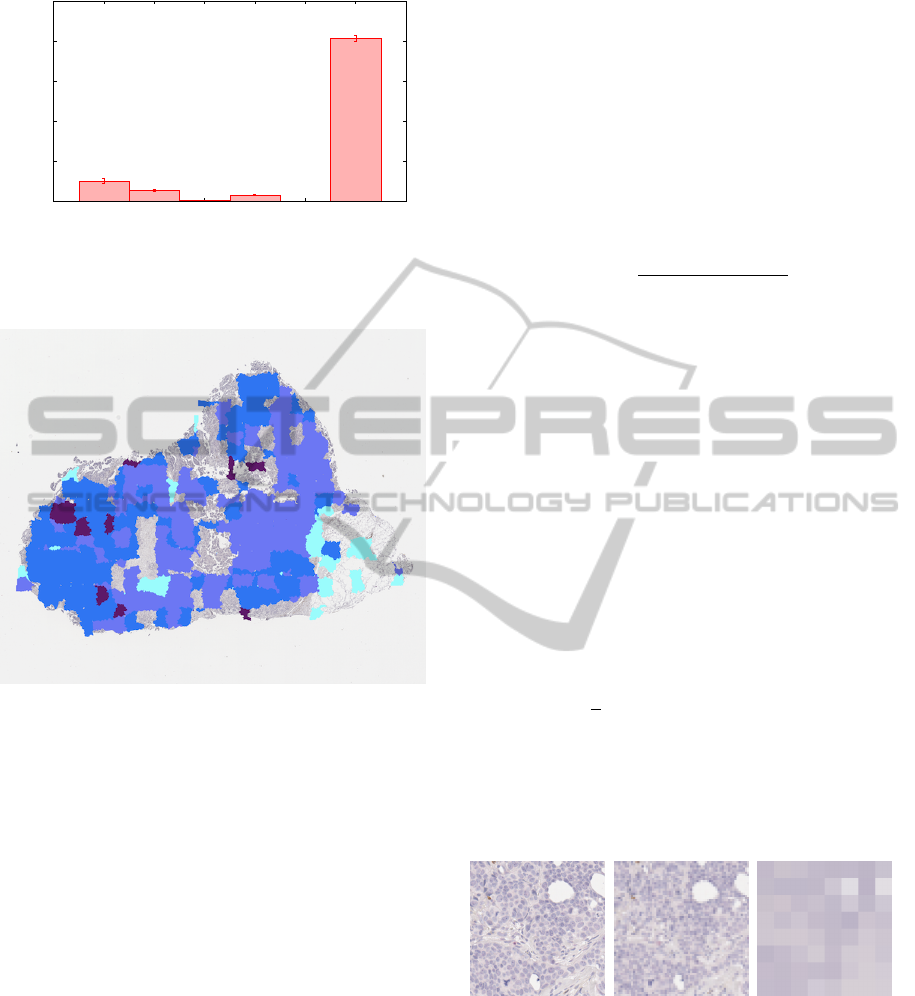
zation, thresholding). Moreover, the classes are not
uniformly represented in our data (Fig. 13): while ex-
cluded elements are described by only a handful of
annotations, they actually account for the majority of
the area of the images, especially because of the back-
VISAPP2014-InternationalConferenceonComputerVisionTheoryandApplications
314
0
0.2
0.4
0.6
0.8
1
Diffuse
Solid
DCIS
Stroma
Nonneoplastic
Excluded
AREA
Figure 13: Relative areas of all the classes: average for each
training set. Standard deviation is given as vertical bars.
Figure 14: Classification map obtained by the presented
method; the colors match those used by the expert, except
for the excluded regions which are left untouched.
ground; on the other hand, ductal structures constitute
a minority and are sometimes completely missing.
Nonetheless, the delimited regions appear to ex-
hibit a texture-related behavior, and we can use that
to decide on a model: a delimited region is made of
a set of patches that can be identified by their texture,
and delimited regions of the same class share the same
set of textures. Thus, by partitioning the image into
patches and labeling each patch based on its texture,
we can draw a color-coded map like in Fig. 14.
We already expected that some classes (ductal
structures) would be difficult to distinguish with only
texture information. But if the image can be decom-
posed into identifiable blocks, then it might be possi-
ble in future work to perform morphology-based anal-
ysis without the need for precise cell segmentation,
giving a general framework to describe the contents of
a histopathological image, regardless of the cell con-
tents of the studied classes.
4.2 Model Evaluation
The method is evaluated with a leave-one-out cross-
validation involving all the annotated images: for
each image (in our set of 7), a training base is created
with the other 6. All the values given in the rest of
this article are obtained by averaging the values from
7 experiments.
The quality of the model can be measured by com-
puting the certainty of the training base for each label
l:
C(l) =
|B
−1
({l})|
|{t ∈ T : l ∈ B(t)}|
(4)
When the certainty is 100%, it means that the only
group containing the label is a singleton, and so the
textures can be used to uniquely characterize the cor-
responding class. On the other hand, a certainty of
0% means that the textures are too ambiguous for a
one-to-one mapping.
Since a human pathologist uses a multi-resolution
approach (Roullier et al., 2011), a whole slide image
is typically provided as a set of images corresponding
to different magnifications that can be used by visual-
ization software to speed up display. But they restrict
the systematic study of the impact of the resolution
level, and can also cause additional degradation due
to lossy compression. So, in order to determine the
information available at each level of detail (LOD),
we compute for each image I a pyramid defined by:
I
LOD
(x,y) =
1
4
∑
(i, j)∈{0,1}
2
I
LOD−1
(2x + i, 2y + j) (5)
The original image is at LOD 0 (Fig. 15). It can be
observed that high resolution is correlated with high
data set certainty for the chosen texture descriptor
(Fig. 16).
(a) LOD 0 (b) LOD 3 (c) LOD 6
Figure 15: Visualization of the effect of the resolution pa-
rameter LOD on pixel data.
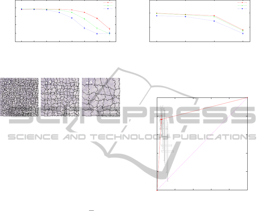
Ideally, the segmentation algorithm should create
patches of the right size, so that each patch would
contain just enough information to identify a class-
characteristic texture. Instead, we will assume the ex-
istence of a common texture scale that applies to all
classes: the segmentation parameter S (Fig. 17). At
high resolution, a texture described by its color can
FastSegmentationforTexture-basedCartographyofwholeSlideImages
315
0.6
0.7
0.8
0.9
1
0 1 2 3 4 5 6 7
C
LOD
All
S 8
S 16
S 32
Figure 16: Visualization of the effect of the resolution pa-
rameter LOD on the overall certainty of the training base
for different values of S and Q = 4. Standard deviation is
given as vertical bars.
(a) S 8 (b) S 16 (c) S 32
Figure 17: Visualization of the effect of the segmentation
parameter S on patch generation.
help identify a class with very little doubt (Fig. 16).
But at lower resolutions, larger values of S increase
the ambiguity of the texture description, because the
patches become large enough to contain multiple tex-
tures from adjacent regions of different classes.
Finally, despite the use of sparse structures, a one
nearest neighbor classification using color histograms
requires large amounts of memory and processing
time. A simple yet effective technique to mitigate
this issue is to use a quantization scheme where the
values used as histogram keys are 2
Q
b
v
2
Q
c instead of
v, and Q is the quantization parameter. Less mem-
ory is required because textures with close descrip-
tors are merged. As Fig. 18 shows, a mild quantiza-
tion (Q ≤ 4) barely affects the certainty of the training
base.
By considering only this measure of the train-
ing base quality, we would expect to get the best re-
sults with high resolution, small patches and minimal
quantification. But we experimentally determined
that the configuration (LOD 4, Q 4, S 32) yielded the
best overall outcome when plotting the data in ROC
space (Fig. 19). The discrepancy between high train-
ing base certainty and lesser classification results can
have several causes, explored in the next section.
4.3 Classification Results
By observing the confusion matrix for a chosen set
of parameters (table 2), we can see that the class of
the excluded regions is the only one to be adequately
detected.
0.8
0.9
1
0 2 4 6
C
Q
All
S 8
S 16
S 32
Figure 18: Visualization of the effect of the quantization
parameter Q on the overall certainty of the training base
for different values of S and LOD = 4. Standard devia-
tion is given as vertical bars (barely visible because they
are small).
0
0.2
0.4
0.6
0.8
1
0 0.2 0.4 0.6 0.8 1
TPR
FPR
All
LOD4 Q4 S32
Figure 19: ROC points (light gray) for each parameteriza-
tion are obtained by merging experimental data points for
all the classes. For clarity, a convex curve (red) has been
synthesized from these points with one point that stands out;
such a synthetic curve makes sense because a classifier can
be built for any interpolated point (Fawcett, 2006). Standard
deviation is given as horizontal and vertical bars.
The ductal structures of the DCIS class are diffi-
cult to identify because of their ambiguous textures,
but also because of their rarity. Surprisingly, the non-
neoplastic ductal structures seem more prone to tex-
tural characterization, but the values are inconclusive
due to the high standard deviation caused by the rar-
ity of the class and the small number of annotated im-
ages.
The remaining 3 classes illustrate some limita-
tions of the model. The ”stroma” class is detected
as ”excluded regions”, ”stroma” and ”diffuse inva-
sion”. As it turns out, ”diffuse invasion” means that
textures corresponding to cancerous cells are mixed
with textures corresponding to stroma. This mixing
creates conflicts which are resolved by assigning the
VISAPP2014-InternationalConferenceonComputerVisionTheoryandApplications
316

Table 2: Confusion matrix for a particular parameterization (LOD 4, Q 4, S 32). Results are given as mean and standard
deviation computed from 7 values.
DCIS
Excluded
regions
Stroma
Solid
formations
Nonneoplastic
objects
Diffuse
invasion
DCIS
57% ± 49 29% ± 35 2% ± 5 4% ± 4 0.1% ± 0.2 8% ± 10
Excluded
regions
0.3% ± 0.4 85% ± 3 3% ± 1 3% ± 2 0.2% ± 0.2 9% ± 3
Stroma
1% ± 3 29% ± 10 31% ± 10 4% ± 3 0.1% ± 0.2 25% ± 10
Solid
formations
0.9% ± 2 19% ± 14 0.5% ± 0.6 44% ± 32 0.0% ± 0.1 35% ± 24
Nonneoplastic
objects
0% ± 0 11% ± 20 0.6% ± 1 6% ± 14 71% ± 45 12% ± 18
Diffuse
invasion
0.2% ± 0.2 37% ± 12 3% ± 3 11% ± 9 2% ± 3 47% ± 15
”excluded regions” class to the ambiguous textures
(section 3.3). The same phenomenon explains why
both ”solid formations” (regions of high cancerous
cell density) and ”diffuse invasion” (regions of low
cancerous cell density) are detected as a mixture of
”excluded regions”, ”solid formations” and ”diffuse
invasion”. The pathologist who made the annotations
told us that the difference between ”solid formation”
and ”diffuse invasion” can be debatable. So, by merg-
ing these 2 classes, we could get a much higher detec-
tion rate (possibly up to 90%).
But the underlying problem is that the model is
flawed: a texture unit defined by one patch is not
enough to identify a class. The certainty of the train-
ing bases is high because, unexpectedly, simple color
histogram are not only strong enough to describe such
texture units, but they also capture small variations
that can almost identify the patches themselves, hence
the large size of the training bases (see next sec-
tion). The images are mostly ”clean”, the only visu-
ally (barely) noticeable noise seeming to be compres-
sion artifacts (lossy JPEG2000). So these variations
are more likely a “content noise”, a mix of a variety of
biological and nonbiological elements. When used to
analyze a new image, these small variations give way
to the main constituents of the texture. We conjecture
that if we could remove these variations, we would
obtain a small set of textures (maybe a few dozens)
that could be used to identify regions like a pathol-
ogist does. With that in mind, the confusion matrix
could suggest that regions corresponding to stroma,
diffuse invasion and solid formations are made up of
the same set of textures (as described by color his-
tograms of patches), but they differ by the proportions
of these textures; that phenomenon could be quanti-
fied by measuring their local density distributions.
Another clue in support of that conjecture is the
specificity data (table 3). While the presence of a
given texture is not always enough to identify only
one given class, its presence might still be a necessity
and thus its absence can reliably be used to exclude
some classes, especially for stroma (sparsely popu-
lated regions with a “sinuous” appearance) and solid
formations (dense clumps of large cancerous cell nu-
clei). The specificity for the excluded regions is lower
because of its role as “default class” to resolve ambi-
guities in our current method, as explained previously.
At this time, we believe that we don’t have enough
data on DCIS and nonneoplastic objects to draw a def-
inite conclusion on these classes.
4.4 Performance
The experiments were run on an AMD Opteron 2
GHz with 32 Gb of memory. The segmentation step
takes at most a few minutes even on large images (less
than 2 minutes for a full gigapixel image with our cur-
rent sequential Java implementation). But, as shown
on Fig. 20, the main bottleneck of the method is the
size of the training bases, mostly because of the time
needed to search a nearest neighbor. So far, this has
prevented us from testing our current algorithm with
high resolutions but we have verified that capping the
training base size to 10000 elements (which is still
large) can bring down the computing time to less than
2 hours for the highest resolution. That being said,
our current results suggest that lower resolutions may
already have enough information to completely ana-
FastSegmentationforTexture-basedCartographyofwholeSlideImages
317
Table 3: Sensitivity and specificity for a particular param-
eterization (LOD 4, Q 4, S 32). Results are given as mean
and standard deviation computed from 7 values.
Class Sensitivity Specificity
DCIS
57% ± 49 99.6% ± 0.6
Excluded
regions
85% ± 3 67% ± 13
Stroma
31% ± 10 97% ± 2
Solid
formations
44% ± 32 96% ± 3
Nonneoplastic
objects
71% ± 45 99.8% ± 0.2
Diffuse
invasion
47% ± 15 89% ± 4
lyze the image.
10
0
10
1
10
2
10
3
10
4
10
5
10
2
10
3
10
4
10
5
10
6
TIME (s)
ENTRIES
LOD 7
LOD 6
LOD 5
LOD 4
LOD 3
Figure 20: Mean sequential calculation time by image ac-
cording to the size of the training base. Each point corre-
sponds to a setting (LOD, Q) for a segmentation of size 32
pixels. The colored discs symbolize the image size, related
to the parameter LOD. Some experiments at high resolution
were not performed because of excessive time and memory
requirements. Standard deviation is given as horizontal and
vertical bars.
5 CONCLUSIONS AND FUTURE
WORK
The recent advent of whole slides images is a great
opportunity to provide new diagnostic tools and to
help pathologists in their clinical analyses. However,
it also comes with great challenges, mainly due to the
large size of the images and the complexity of their
content. To achieve a fast and efficient classification
of the images, we proposed in this paper a methodol-
ogy enabling to partition the initial image in relevant
regions. This approach is based on an original seg-
mentation algorithm and on a supervised classifica-
tion using a textural characterization of each region.
We carried out experiments on 7 annotated images
and obtained promising results. In the future, we are
planning to analyze the images at a lower level in or-
der to detect each single cell and complex biological
structures present in the images. We believe that iden-
tifying theses structures and being able to accurately
classify them is the key to the development of future
clinical tools. Furthermore, it will help to improve the
development of patient-specific targeted treatment.
REFERENCES
Elston, C. W. and Ellis, I. O. (1991). Pathological prognos-
tic factors in breast cancer. i. the value of histological
grade in breast cancer: Experience from a large study
with long-term follow-up. Histopathology.
Fawcett, T. (2006). An introduction to roc analysis. Pattern
Recognition Letters.
Ghaznavi, F., Evans, A., Madabhushi, A., and Feldman, M.
(2013). Digital imaging in pathology: Whole-slide
imaging and beyond. Annual Review of Pathology.
Gurcan, M. N., Boucheron, L. E., Can, A., Madabhushi, A.,
Rajpoot, N. M., and Yener, B. (2009). Histopatho-
logical image analysis: a review. IEEE Reviews in
Biomedical Engineering.
Homeyer, A., Schenk, A., Arlt, J., Dahmen, U., Dirsch, O.,
and Hahn, H. K. (2013). Practical quantification of
necrosis in histological whole-slide images. Comput-
erized Medical Imaging and Graphics.
Huang, C.-H., Veillard, A., Roux, L., Lom
´
enie, N., and
Racoceanu, D. (2010). Time-efficient sparse analysis
of histopathological whole slide images. Computer-
ized Medical Imaging and Graphics.
Montanari, U. (1971). On the optimal detection of curves
in noisy pictures. Communications of the ACM.
Ojala, T., Pietik
¨
ainen, M., and Harwood, D. (1996). A com-
parative study of texture measures with classification
based on featured distributions. Pattern Recognition.
Roullier, V., L
´
ezoray, O., Ta, V.-T., and Elmoataz, A.
(2011). Multi-resolution graph-based analysis of
histopathological whole slide images: application to
mitotic cell extraction and visualization. Computer-
ized Medical Imaging and Graphics.
Ruiz, A., Sertel, O., Ujaldon, M., Catalyurek, U., Saltz, J.,
and Gurcan, M. (2007). Pathological image analy-
sis using the gpu: Stroma classification for neuroblas-
toma. 2007 IEEE International Conference on Bioin-
formatics and Biomedicine (BIBM 2007).
Sertel, O., Kong, J., Shimada, H., and Catalyurek, U.
(2009). Computer-aided prognosis of neuroblastoma
on whole-slide images: Classification of stromal de-
velopment. Pattern Recognition.
VISAPP2014-InternationalConferenceonComputerVisionTheoryandApplications
318

Signolle, N., Plancoulaine, B., Herlin, P., and Revenu, M.
(2008). Texture-based multiscale segmentation: Ap-
plication to stromal compartment characterization on
ovarian carcinoma virtual slides. Image and Signal
Processing.
Tavassoli, F. A. and Devilee, P. (2003). Pathology and Ge-
netics of Tumours of the Breast and Female Genital
Organs. IARCPress.
Wemmert, C., Kr
¨
uger, J., Forestier, G., Sternberger, L.,
Feuerhake, F., and Ganc¸arski, P. (2013). Stain unmix-
ing in brightfield multiplexed immunohistochemistry.
IEEE International Conference on Image Processing.
FastSegmentationforTexture-basedCartographyofwholeSlideImages
319
