
Automatic Generation of Structural Building Descriptions
from 3D Point Cloud Scans
Sebastian Ochmann
1
, Richard Vock
1
, Raoul Wessel
1
, Martin Tamke
2
and Reinhard Klein
1
1
Institute of Computer Science II, University of Bonn, Bonn, Germany
2
Centre for Information Technology and Architecture (CITA), The Royal Danish Academy of Fine Arts,
School of Architecture, Copenhagen, Denmark
Keywords:
Scene Understanding, Building Structure, Point Cloud, Laser Scanning, Segmentation.
Abstract:
We present a new method for automatic semantic structuring of 3D point clouds representing buildings. In
contrast to existing approaches which either target the outside appearance like the facade structure or rather
low-level geometric structures, we focus on the building’s interior using indoor scans to derive high-level
architectural entities like rooms and doors. Starting with a registered 3D point cloud, we probabilistically
model the affiliation of each measured point to a certain room in the building. We solve the resulting clustering
problem using an iterative algorithm that relies on the estimated visibilities between any two locations within
the point cloud. With the segmentation into rooms at hand, we subsequently determine the locations and
extents of doors between adjacent rooms. In our experiments, we demonstrate the feasibility of our method by
applying it to synthetic as well as to real-world data.
1 INTRODUCTION
Digital 3D representations of buildings highly dif-
fer regarding the amount of inherent structuring. On
the one hand, new building drafts are mainly created
using state-of-the-art Building Information Modeling
(BIM) approaches that naturally ensure a high amount
of structuring into semantic entities ranging e.g. from
storeys and rooms over walls down to doors and win-
dows. On the other hand, 3D point cloud scans, which
today are increasingly used as a documentation tool
for already existing, older buildings, are almost com-
pletely unstructured. The semantic gap between such
low- and high-level representations hinders the effi-
cient usage of 3D point cloud scans for various pur-
poses including retrofitting, renovation, and semantic
analysis of the legacy building stock, for which no
structured digital representations exist. As a solution,
architects and construction companies usually use the
measured point cloud data to manually generate a 3D
BIM overlay that provides enough structuring to al-
low easy navigation and computation of key proper-
ties like room or window area. However, this task is
both cumbersome and time-consuming.
While existing approaches for building structuring
either require 3D CAD models (Wessel et al., 2008;
Langenhan et al., 2012), consider primarily outdoor
(airborne) scans (Verma et al., 2006; Schnabel et al.,
2008; Bokeloh et al., 2009), or target the recogni-
tion of objects like furniture inside single rooms (Kim
et al., 2012; Nan et al., 2012), our method focuses on
the extraction of the overall room structure from in-
door 3D point cloud scans. We aim at first decompos-
ing the point cloud such that each point is assigned to
a room. To this end, we propose a probabilistic clus-
tering algorithm that exploits knowledge about the be-
longing of each measured point to a particular scan.
The resulting segmentation constitutes the fundamen-
tal building block for computing important key prop-
erties like e.g. room area. In a second step we detect
doors connecting the rooms and construct a graph that
encodes the building topology.
Our method may be summarized as follows (see
also Figure 1): We start with multiple indoor 3D point
clouds scans which have been registered beforehand
(this step is not in the scope of this paper). Each
point is initially labeled with an index of the scan from
which it originates. In a preprocessing step, normals
are estimated for each point (if necessary) and planar
structures are detected using the algorithm by (Schn-
abel et al., 2007). This yields a set of planes together
with subsets of points corresponding to each plane.
Next, point sets belonging to scanning positions that
are located in the same room are merged; this affects
120
Ochmann S., Vock R., Wessel R., Tamke M. and Klein R..
Automatic Generation of Structural Building Descriptions from 3D Point Cloud Scans.
DOI: 10.5220/0004689601200127
In Proceedings of the 9th International Conference on Computer Graphics Theory and Applications (GRAPP-2014), pages 120-127
ISBN: 978-989-758-002-4
Copyright
c
2014 SCITEPRESS (Science and Technology Publications, Lda.)
41.16m
2
48.16m
2
108.44m
2
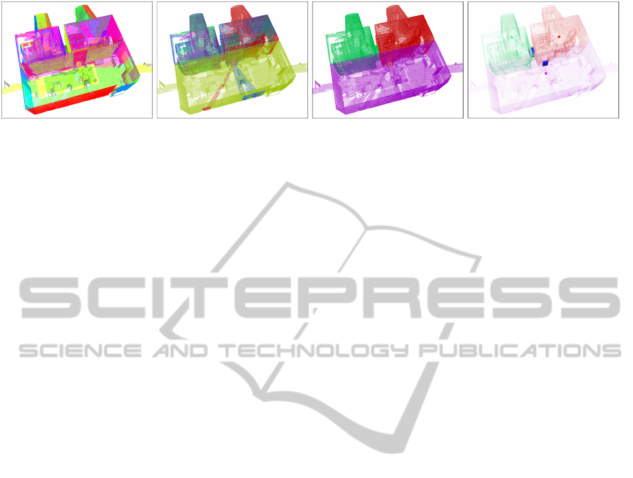
Figure 1: Overview of our method. From left to right: Detected planar structures; colour-coded indices of the individual
scans; final point assignments after the re-labeling process; extracted room topology graph.
those rooms in which scans from multiple positions
were performed. This step may be either performed
automatically or semi-automatically using a graphical
user interface for correcting automatically generated
results. Following the merging step, an iterative re-
labeling process is performed to update assignments
of points to rooms. This process uses a probabilistic
model to estimate updated soft assignments of points
to room labels. After convergence, a new (hard) as-
signment of points to rooms is obtained.
Finally, the original and the new labeling of the
points are used to determine the locations and extents
of doors between pairs of adjacent rooms. Together
with the set of room points, this constitutes a room
connectivity graph in which rooms are represented by
attributed nodes and doors are represented by edges.
Such representations are an important tool for seman-
tic building analysis or graph-based building retrieval
(Wessel et al., 2008; Langenhan et al., 2012).
The contributions of this paper are:
1. Automatic decomposition of a 3D indoor building
scan into rooms.
2. A method for detecting connections between ad-
jacent rooms using the computed decomposition.
3. Construction of a graph encoding the building’s
topology purely from point clouds.
2 RELATED WORK
In this Section we briefly review the related work on
the extraction of structural building information from
digital representations.
2.1 Point-cloud-based Approaches
In (Verma et al., 2006) a parametric shape grammar
is used to detect common roof shapes in LIDAR data.
They initially extract connected components of pla-
nar point sets and filter out small components in order
to get separated subsets of points for ground and roof
structures. Subsequently arbitrary polygons are fitted
to the roof and by analyzing their topological rela-
tions, simple, parameterized roof shapes are matched
to the scan data. This approach is rather specific
to roof shape detection, where a concise, parametric
model for detected objects can be derived. By rep-
resenting point clouds as a topology graph of inter-
related basic shape primitives (Schnabel et al., 2008)
reduce the problem of finding shapes in point clouds
to a subgraph matching problem. The scene as well
as the query object are decomposed into primitive
shapes using a RANSAC (random sample consensus)
approach. A topology graph for each cloud is con-
structed capturing the spatial relationships between
these primitive shapes. A lot of research has recently
been conducted in exploiting symmetries in order to
understand scan data. For example (Bokeloh et al.,
2009) detect partial symmetries in point cloud data by
matching line features detected using slippage analy-
sis of point neighbourhoods in a moving least squares
scheme. Matching these line features and extracting
symmetric components yields a decomposition of the
scanned scene into cliques of symmetric parts. These
parts however do not necessarily carry a semantic
meaning in architectural terms and are therefore not
suited for semantic analysis of building structures.
While the above methods are used to structure
scans showing the outside of a building, the interior of
buildings has recently gained attention, especially in
the field of robotics, where segmentation of furniture
is an important topic for indoor navigation, see e.g.
(Rusu et al., 2008; Koppula et al., 2011). An itera-
tive search-and-classify method is used by (Nan et al.,
2012) for segmentation of indoor scenes. They start
with an over-segmented scene and iteratively grow re-
gions while maximizing classification likelihood. A
similar, supervised learning approach is used by (Kim
et al., 2012). Their method is divided into a learn-
ing phase, in which multiple scans of single objects
are processed in order to obtain a decomposition into
simple parts as well as to derive their spatial relations,
and a recognition phase. Both of these methods focus
on the recognition of objects like furniture that can be
well represented by certain templates and do not take
the overall room structure of a building into account.
AutomaticGenerationofStructuralBuildingDescriptionsfrom3DPointCloudScans
121

2.2 Approaches based on Alternative
Representations
(Wessel et al., 2008) extract topological information
from low-level 3D CAD representations of buildings.
They find floor planes in the input polygon soup and
extract 2D plans by cutting each storey at different
heights. These cuts are then analyzed in order to
extract rooms and inconsistencies between different
cut heights yield candidates for doors and windows.
In (Langenhan et al., 2013), high-level BIM models
are used for the extraction of a building’s topology.
They derive information about the topological rela-
tionship between rooms from IFC (Industry Founda-
tion Classes) files by analysis of certain entity con-
stellations which can be used to perform sketch-based
queries in a database. (Ahmed et al., 2012) use 2D
floor plans to extract the structure and semantics of
buildings. The input drawing is first segmented into
graphical parts of differing line thickness used to ex-
tract the geometry of rooms by means of contour de-
tection and symbol matching, and a textual part used
for semantic enrichment by means of OCR (optical
character recognition) and subsequent matching with
predefined room labels. A hybrid approach is pre-
sented in (Xiao and Furukawa, 2012). The authors use
3D point cloud data together with ground-level pho-
tographs to reconstruct a CSG representation based on
fitted rectangle primitives. Note that this work rather
focuses on indoor scene reconstruction than on the ac-
tual extraction of a semantic structuring.
3 PREPROCESSING
The input data for our method consists of multiple
3D point clouds which have been registered before-
hand in a common world coordinate system. The reg-
istration step is usually done automatically or semi-
automatically by the scanner software and is not in
the scope of this paper. Each individual scan also con-
tains the scanner position.
If normals are not part of the input data, they are
approximated by means of local PCA (principal com-
ponent analysis) of point patches around the individ-
ual data points. To determine the correct orientation
of the normal, it is checked whether the determined
normal vector points into the hemisphere in which the
scanner position associated with the point is located.
Subsequently, planar structures are detected in the
whole point cloud using a RANSAC algorithm by
(Schnabel et al., 2007). This yields a set of planes de-
fined by their normal and distance to the origin. Addi-
tionally, the association between each plane p ∈P and
the point set P
p
that constitutes this plane is stored.
The known assignments of points to the individ-
ual scans will be used in the next section as an initial
guess which points belong to a room. As one par-
ticular room may have been scanned from more than
one scanner location, scans belonging to the same
room are merged. This step is performed in a semi-
automatic manner. A conservative measure whether
two scans belong to the same room is used to give
the user suggestions which scans should be merged.
This measure takes into account the ratio of overlap-
ping points between two scans to the total number of
involved points. If the ratio is above a certain thresh-
old, the rooms are suggested to be merged. The user
may choose to accept these suggestions or make man-
ual changes as desired. Note that the original scanner
positions are stored for later usage, together with the
information which scans were merged.
4 PROBABILISTIC
POINT-TO-ROOM LABELING
After the merging step described in Section 3, we are
left with m different room labels and their associated
points. In the following, we describe the task of point-
to-room assignment as a probabilistic clustering prob-
lem (Duda et al., 2001). Let ω
j
, j = 1, ..., m denote
the random variable that indicates a particular room,
and furthermore, let x denote a random variable corre-
sponding to a point in R
3
. Then the class-conditional
densities p(x|ω
j
) describe the probability for observ-
ing a point x given the existence of the jth room. By
that, we can describe the problem of segmenting a
point cloud into single rooms by computing the con-
ditional probability p(ω
j
|x) that an observed point x
belongs to the jth room. Given a particular observa-
tion x
k
from the point cloud scan, we can determine
its probabilistic room assignment by computing
p(ω
j
|x
k
) =
p(x
k
|ω
j
)p(ω
j
)
∑
m
j
0
=1
p(x
k
|ω
j
0
)p(ω
j
0
)
. (1)
From the above equation it becomes clear that de-
termining the clustering actually boils down to model-
ing and computing the class-conditional probabilities.
Intuitively speaking, for a particular room p(x
k
|ω
j
)
should provide a high value if the observed measure-
ment x
k
lies inside it. Suppose we already knew a set
of points X
j
that belongs to the room. A good choice
to decide whether an observation lies inside would be
to consider the visibility v
j
(x
k
) ∈[0, 1] of this particu-
lar point from all the other points in X
j
that we know
belong to the room (we will describe how to estimate
the visibility in detail in Section 5).
GRAPP2014-InternationalConferenceonComputerGraphicsTheoryandApplications
122
In order to steer the impact of varying visibili-
ties we formulate the class-conditional probability in
terms of a normal distribution over the visibilities:
p(x
k
|ω
j
, σ) =
1
√
2πσ
2
exp
−
(1 −v
j
(x
k
))
2
2σ
2
!
. (2)
Apparently, computing the visibility v
j
(x
k
) re-
quires knowledge about the exact dimensions of the
room, rendering the underlying clustering a chicken-
egg problem. We alleviate by starting with an ed-
ucated guess about the point-to-room assignments,
which is given by the information which points orig-
inate from the individual (merged) scans. This prior
knowledge is used to compute v
j
(x
k
) in the first it-
eration. We then iterate between the cluster assign-
ment and visibility computation until our algorithm
converges. In Algorithm 1, we show an overview of
the iterative assignment process.
Data: A set of observations x
k
∈ R
3
, k = 1, ..., n
Data: A set of initial room assignments:
∀ k ∃ r
init
(x
k
) ∈ {1, ..., m}
Data: A set of planes p
i
∈ P , i = 1, ..., |P |
Result: A new point-to-room assignment:
∀ k ∃ r
f inal
(x
k
) ∈ {1, ..., m}
Initialize prior room probabilities according to
number of measured points:
p(ω
j
) :=
|{r
init
(x
k
)= j,k=1,...,n}|
∑
m
j
0
=1
|{r
init
(x
k
)= j
0
,k=1,...,n}|
;
Initialize r
curr
(x
k
) := r
init
(x
k
);
while not converged do
Compute the set of points belonging to the
jth room: X
j
:= {x|r
curr
(x) = j};
Compute class-conditional probabilities:
p(x
k
|ω
j
, σ) :=
1
√
2πσ
2
exp
−
(
1−v
j
(x
k
)
)
2
2σ
2
;
Compute probabilistic cluster assignments:
p(ω
j
|x
k
) =
p(x
k
|ω
j
)p(ω
j
)
∑
m
j
0
=1
p(x
k
|ω
j
0
)p(ω
j
0
)
;
Compute hard cluster assignments:
r
curr
(x
k
) = argmax
j=1,...,m
p(ω
j
|x
k
);
Renormalize room priors:
p(ω
j
) :=
1
n
∑
n
k=1
p(ω
j
|x
k
)
end
r
f inal
(x
k
) := r
curr
(x
k
);
Algorithm 1: Iterative room-to-point assignment.
In our tests we use a fixed σ throughout the itera-
tions and for all rooms (see Section 9). Note however
that it might improve results if for each room individ-
ual σ
j
would be used. Estimation of σ
j
and computa-
tion of the soft assignments could be carried out using
an expectation-maximization (EM) algorithm (Demp-
ster et al., 1977).
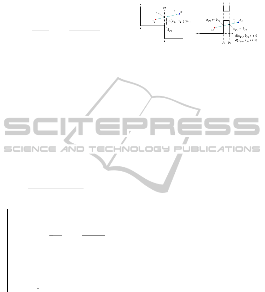
Figure 2: Different cases of visibility estimation. Left: Vis-
ibility between two points x
1
, x
2
located within a room. The
line-of-sight is unobstructed since line segment s does not
intersect any building structure. Right: If a wall lies be-
tween x
1
, x
2
, s intersects multiple planes and visibility is
estimated to be low.
5 VISIBILITY ESTIMATION
We construct the visibility function v
j
(x
k
) to estimate
how unobstructed the line-of-sights between a point
x
k
to all (or a sampled subset of) points X
j
of the jth
room are on average.
The intuition behind this functional is depicted in
Figure 2. If we wish to estimate the visibility between
the points x
1
and x
2
, we take into account the set of
planes p
i
that are intersected by the line segment s
between the two points. For intersection testing, we
consider the complete infinitely large plane. Because
a plane p
i
is only constituted by a subset of the mea-
sured points, the line segment s passing through that
plane shall only be considered to be highly obstructed
if measured points exist in the vicinity of the intersec-
tion point. Let x
p
i
be the intersection point of s with
plane p
i
and let ˆx
p
i
be the point belonging to the plane
p
i
which is closest to x
p
i
:
ˆx
p
i
:= argmin
x∈P
p
||x −x
p
i
||
2
. (3)
The left half of Figure 2 shows the situation that s
is located completely inside a single room. Note that,
in this case, d(x
p
1
, ˆx
p
1
) is large and thus the visibility
regarding plane p
1
is high. In the right half, the sit-
uation of s crossing through a wall is shown. In this
case, the distances d(x
p
1
, ˆx
p
1
) and d(x
p
2
, ˆx
p
2
) to the
nearest points in the planes are (almost) zero and thus
the estimate of the visibility between the points is low.
Let p be a plane and x
p
the intersection of s with
p. Furthermore, for the set of planes P and the set of
all measured points X, let
v
p
(x
1
, x
2
, p) : X ×X ×P → [0, 1] (4)
be a function estimating the visibility between x
1
and
x
2
with respect to a plane p following the above in-
tuition which yields a high value iff the line-of-sight
is unobstructed (see Section 9 for implementation de-
tails).
AutomaticGenerationofStructuralBuildingDescriptionsfrom3DPointCloudScans
123
The visibility term over all planes P which s inter-
sects is defined as
v
P
(x
1
, x
2
) :=
1
1 +
∑
p∈P
(1 −v
p
(x
1
, x
2
, p))
. (5)
Intuitively speaking, the more planes with low vis-
ibility values are encountered along the line segment,
the more the total visibility value decreases. Finally,
we use Equation (5) to define the average visibility
from a point x
k
to a point set X
j
containing points la-
beled to belong to the jth room:
v
j
(x
k
) :=
∑
x∈X
j
v
P
(x
k
, x)
|X
j
|
. (6)
6 DOOR DETECTION
The presence of a door causes the points from one sin-
gle scan to belong to at least two different semantic
rooms. As a consequence, when considering a point
that changed the room assignment during our proba-
bilistic relabeling, the associated ray must have been
shot through a connecting door. We exploit this ob-
servation for our door localization method. Note that
this requires the doors to stand open during the scan-
ning process. This assumption is justified as overlaps
between scans are usually required for registration.
In preparation for door detection, we create a map-
ping of planes to rooms by iterating through the set
of planes and counting the number of points on that
plane that are labeled to be part of the individual
rooms. If the number of points belonging to room r
exceeds a threshold, the plane as well as the subset of
points is assigned to r. This process may also assign
one plane to multiple rooms but its constituting point
set is split among the rooms sharing this plane.
The next step is the generation of candidate point
sets that may constitute the coarse shape of one side of
a door opening. Consider a room r consisting of scan-
ner positions s
0
, . . . , s
n
. We are interested in those rays
going from s
i
through the position of the associated
point p
i
where the labeling of p
i
has changed during
the segmentation step. For each such ray, we check
for intersections with each plane belonging to room r
(Figure 3, left). This yields co-planar point sets which
are stored together with the information which room
s
i
belongs to, which room the point p
i
belongs to and
which plane was intersected (Figure 3, middle).
After the candidates have been constructed, we
split the point sets of each candidate into connected
components. This is necessary if a room pair is con-
nected through multiple doors lying in the same plane.
In a final step, pairs of candidates fulfilling certain
constraints are extracted. The first constraint forces
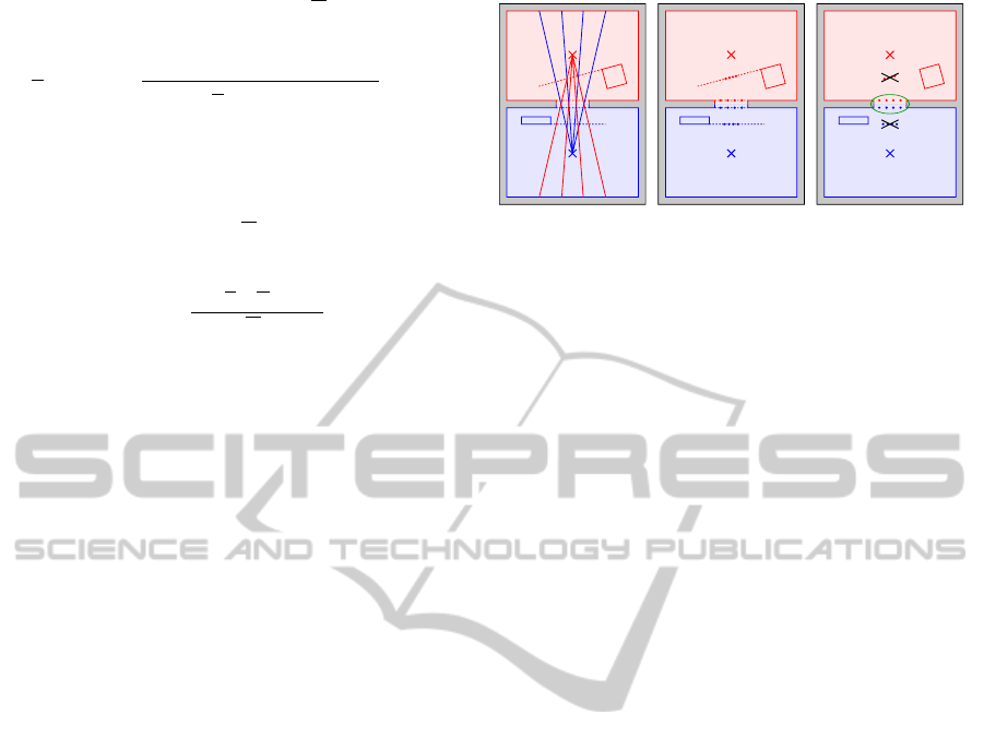
Figure 3: For door detection, the rays whose target point’s
labeling has changed during segmentation are intersected
with the planes belonging to the room in which the scanner
is located (left); the intersection point sets on each plane are
potential door candidates (middle); pairs of candidates that
fulfill certain constraints are extracted (right).
the normals of the two involved planes to point away
from each other. The second constraint forces the dis-
tance between the planes to be within a given range.
Lastly, the point set of one of the candidates is pro-
jected onto the plane of the other candidate and the
intersection between the projected point sets is com-
puted. If the ratio of the points lying in the intersec-
tion is high enough, the candidate pair is considered
to be a door (encircled points in Figure 3, right).
7 GRAPH GENERATION
To construct a graph encoding the building’s room
topology, each room is represented by a node. An
edge is added for each detected door, connecting the
two associated rooms. We enrich this representa-
tion with node and edge attributes. Each node is as-
signed a position which is set to the location of one
of the involved scanners. Alternatively, the mean of
the positions of all points belonging to the respective
room could be used. However, this does not guaran-
tee that the position lies within the room. Further-
more, each node is assigned an approximate room
area which is computed by projecting all points into
a two-dimensional grid that is aligned with the x-
y-plane. The approximate room area is then esti-
mated by computing the area of cells which contain at
least one point. For each door edge, we compute the
bounding box of the previously generated intersection
points. The edge is then assigned this bounding box
which constitutes an approximation of the door’s po-
sition and shape.
8 EVALUATION
We tested our method on synthetic as well as real-
world datasets. Figure 4 shows a result on synthetic
GRAPP2014-InternationalConferenceonComputerGraphicsTheoryandApplications
124
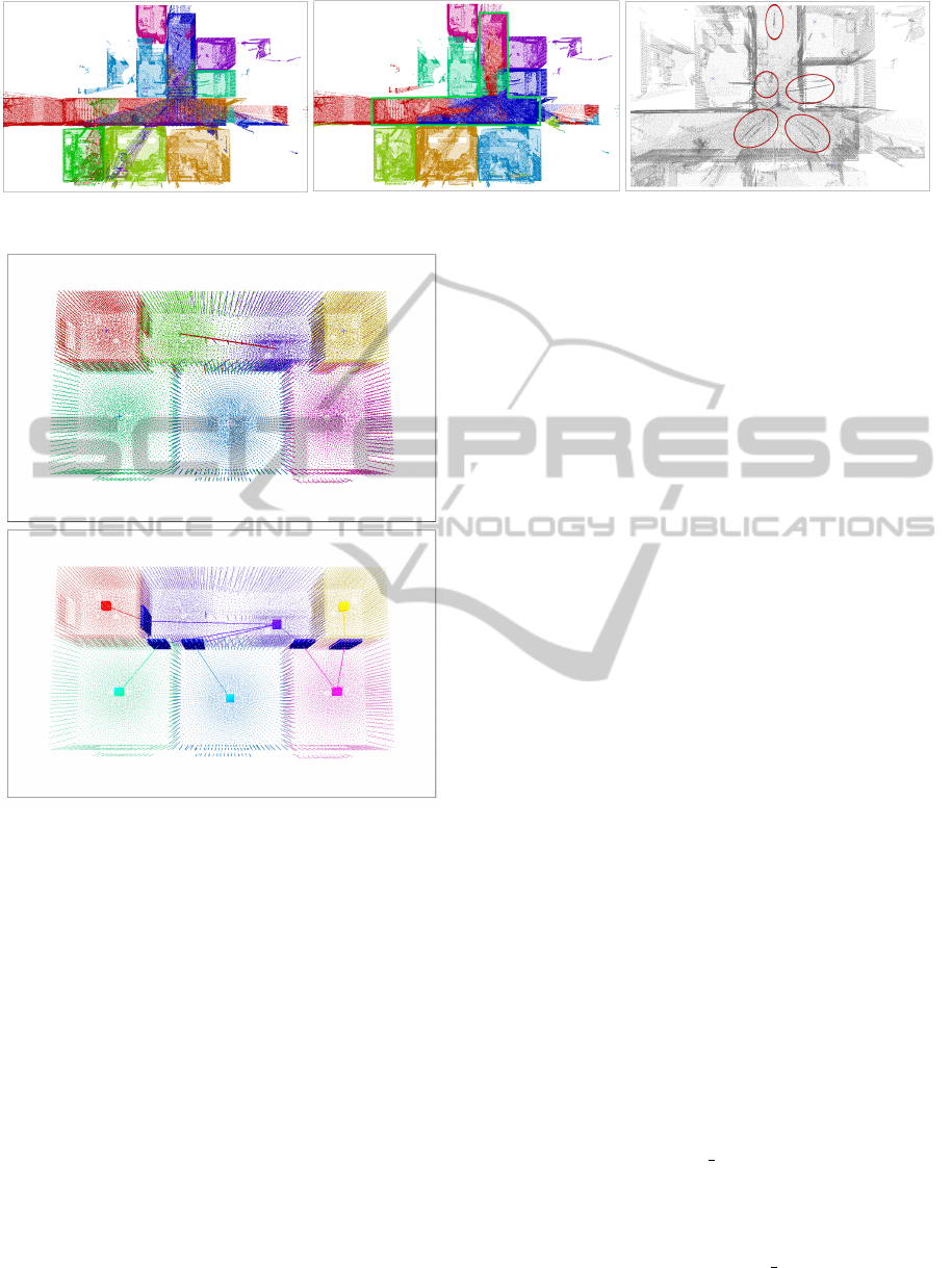
Figure 5: A failure case of our method due to a strongly non-convex room and planar artifacts in the scan data.
8.24m
2
17.16m
2
5.72m
2
17.36m
2
17.28m
2
14.24m
2
Figure 4: Results on synthetic data; the first picture also
shows an automatic merging suggestion (red line between
two scanner positions).
data. In the upper half, the initial labeling of scan
positions is shown, together with an automatically
computed suggestion which scan locations should be
merged (indicated by the red line). The lower half
shows the final topology graph as well as the esti-
mated room areas. Figure 6 shows the results on real-
world data measured in two different storeys of the
same building. The upper-left pictures show the as-
sociation of data points to the individual scans be-
fore merging. On the upper-right, the associations
of points to merged scan positions are shown. The
lower-left part shows the final labeling of the points
after segmentation. The lower-right pictures show
the extracted topology graph including the estimated
room areas as well as the door locations and extents
(blue boxes).
A failure case of our method is shown in Figure
5. The left part shows the initial association to the
scanner positions. In the middle, the labeling after re-
labeling is shown. Many points in the T-shaped cor-
ridor (marked with the green line) were erroneously
labeled to be part of adjacent rooms. The explana-
tion for this behaviour is twofold. Firstly, the as-
sumption that most of the points belonging to a room
can be seen from an arbitrary point within that room
is violated for (strongly) non-convex rooms like the
T-shaped corridor in the depicted dataset. Secondly,
large planar artifacts in the input data (Figure 5, right)
may lead to low visibility values in regions which
should be free space.
Computation time ranges from almost instan-
taneous (for the lower-resolution synthetic dataset
shown in Figure 4 consisting of 70000 points) to
about 30 seconds (for larger datasets as shown in Fig-
ure 6 consisting of about 500000 and 600000 points,
respectively).
9 IMPLEMENTATION DETAILS
For fast determination whether measured points exist
near a point x on a plane p and to enable efficient com-
putations on the GPU, we pre-compute bitmaps for
each plane, providing a discretized occupancy map.
Each pixel may take a continuous value in [0, 1] and
is initially set to 1 if at least one pixel lies within
the boundary of that pixel, and to 0 otherwise. The
bitmaps are subsequently smoothed using a box fil-
ter such that pixels in the vicinity of filled pixels (and
thus points) are assigned values which are negatively
proportional to the distance to the nearest points in the
plane (the distances labeled d(x
p
i
, ˆx
p
i
) in Figure 2).
Using the bitmaps, we approximate the visibility
function v
p
(x
1
, x
2
, p) of Section 5 for two points x
1
, x
2
and a plane p. Let bitmap value
p
(x) be a function of
the plane p’s bitmap value which determines the pixel
value at the projection of x onto p. Then the visibility
function is defined as
v
p
(x
1
, x
2
, p) := 1 −bitmap value
p
(x
p
). (7)
For our experiments, we set σ in Equation 2 to
AutomaticGenerationofStructuralBuildingDescriptionsfrom3DPointCloudScans
125
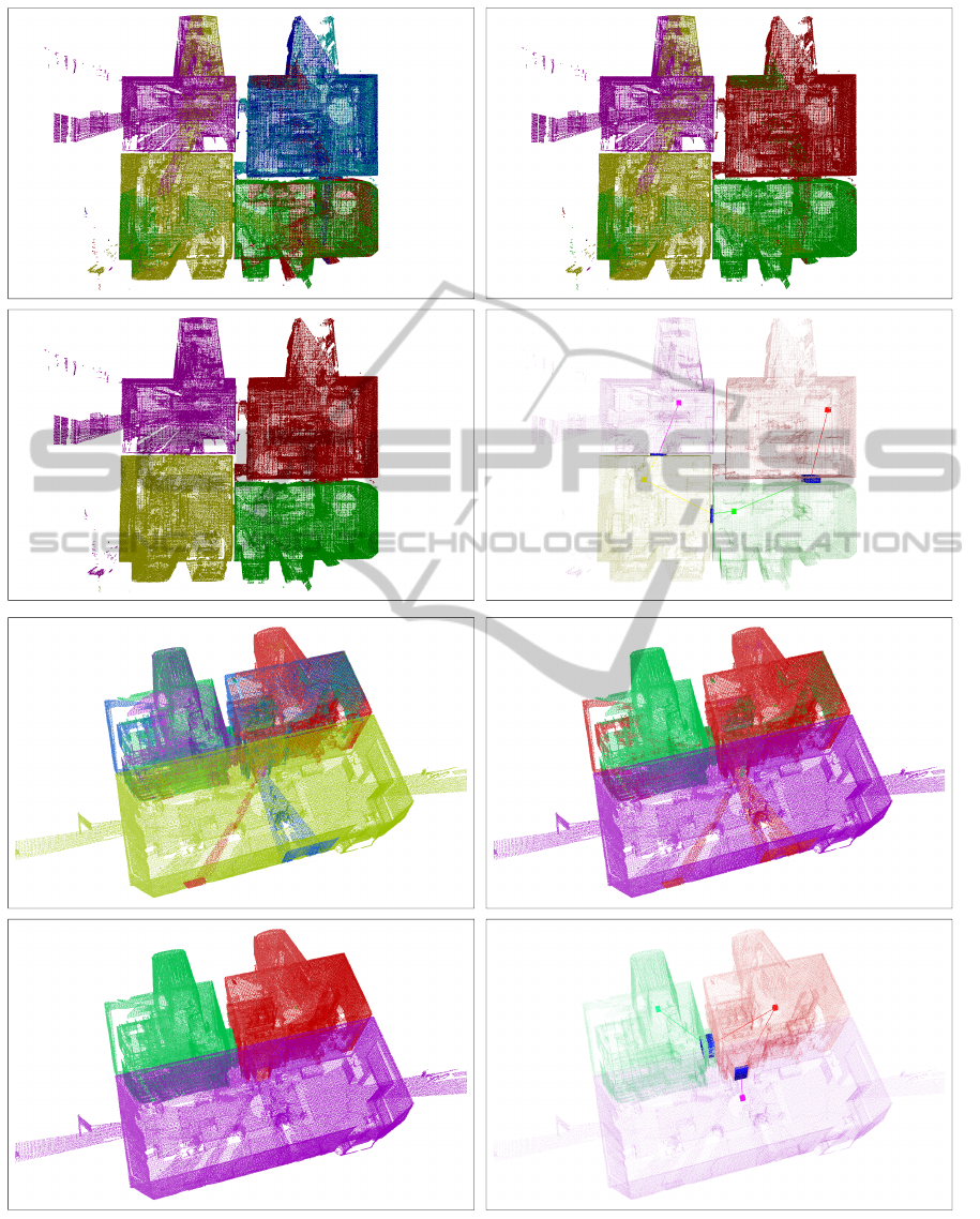
45.72m
2
56.44m
2
43.36m
2
47.24m
2
41.16m
2
48.16m
2
108.44m
2
Figure 6: Results on two real-world datasets. The upper-left pictures show the room associations before merging of scans
belonging to the same rooms. Upper-right: Associations after the merging step. Lower-left: The room assignments after
segmentation. Lower-right: The extracted graphs including detected doors and annotations for the estimated room areas.
GRAPP2014-InternationalConferenceonComputerGraphicsTheoryandApplications
126

0.05. For the plane detection, the minimum count of
points needed to constitute a plane was set to a value
between 200 and 2000, depending on the density of
the dataset. The radius of the box filter for bitmap
smoothing was chosen such that it corresponds to ap-
proximately 20 cm in point cloud coordinates. Visi-
bility tests between pairs of points were computed on
the GPU using OpenCL. The experiments were con-
ducted on a 3.5 GHz Intel Core i7 CPU and a GeForce
GTX 670 GPU with 4 GB of memory. To obtain syn-
thetic data, we implemented a virtual laser scanner
which simulates the scanning process within 3D CAD
building models.
10 CONCLUSIONS AND FUTURE
WORK
We presented a method for the extraction of structural
building descriptions using 3D point cloud scans as
the input data. Our method was evaluated using syn-
thetic and real-world data, showing the feasibility of
our approach. In most cases, the algorithm produced
satisfactory results, yielding useful semantic repre-
sentations of buildings for applications like naviga-
tion in point clouds or structural queries.
The usage of different visibility functionals as
well as an EM-formulation to determine the param-
eters of the used normal distributions separately for
each room label could help to improve the robustness
of our method. Performance in the presence of non-
convex rooms could possibly be improved by using
a measure for (potentially indirect) reachability be-
tween points instead of visibility tests. Also, limiting
the tests to a more local scope may help to overcome
the identified problems. The output of our approach
could be further enriched by more attributes, for in-
stance by applying methods for the analysis of the in-
dividual room point sets after segmentation.
ACKNOWLEDGEMENTS
We would like to thank Henrik Leander Evers for the
scans of Kronborg Castle, Denmark, and the Faculty
of Architecture and Landscape Sciences of Leibniz
University Hannover for providing the 3D building
models that were used for generating the synthetic
data. This work was partially funded by the Euro-
pean Community’s Seventh Framework Programme
(FP7/2007-2013) under grant agreement no. 600908
(DURAARK) 2013-2016.
REFERENCES
Ahmed, S., Liwicki, M., Weber, M., and Dengel, A.
(2012). Automatic room detection and room label-
ing from architectural floor plans. In 10th IAPR In-
ternational Workshop on Document Analysis Systems
(DAS-2012), pages 339–343. IEEE.
Bokeloh, M., Berner, A., Wand, M., Seidel, H.-P., and
Schilling, A. (2009). Symmetry detection using line
features. Computer Graphics Forum (EG 2009),
28(2):697–706.
Dempster, A. P., Laird, N. M., and Rubin, D. B. (1977).
Maximum likelihood from incomplete data via the em
algorithm. JOURNAL OF THE ROYAL STATISTICAL
SOCIETY, SERIES B, 39(1):1–38.
Duda, R., Hart, P., and Stork, D. (2001). Pattern Classifica-
tion. Wiley.
Kim, Y. M., Mitra, N. J., Yan, D.-M., and Guibas, L. (2012).
Acquiring 3d indoor environments with variability
and repetition. ACM TOG, 31(6):138:1–138:11.
Koppula, H. S., Anand, A., Joachims, T., and Saxena, A.
(2011). Semantic labeling of 3d point clouds for in-
door scenes. In NIPS 2011, pages 244–252.
Langenhan, C., Weber, M., Liwicki, M., Dengel, A., and
F., P. (2012). Topological query on semantic building
models using ontology and graph theory. In EG-ICE.
TUM.
Langenhan, C., Weber, M., Liwicki, M., Petzold, F., and
Dengel, A. (2013). Graph-based retrieval of build-
ing information models for supporting the early de-
sign stages. Advanced Engineering Informatics.
Nan, L., Xie, K., and Sharf, A. (2012). A search-classify ap-
proach for cluttered indoor scene understanding. ACM
TOG, 31(6):137:1–137:10.
Rusu, R. B., Marton, Z. C., Blodow, N., Dolha, M., and
Beetz, M. (2008). Towards 3D point cloud based ob-
ject maps for household environments. Robotics and
Autonomous Systems, 56(11):927941.
Schnabel, R., Wahl, R., and Klein, R. (2007). Efficient
ransac for point-cloud shape detection. Computer
Graphics Forum, 26(2):214–226.
Schnabel, R., Wessel, R., Wahl, R., and Klein, R. (2008).
Shape recognition in 3d point-clouds. In WSCG 2008.
UNION Agency-Science Press.
Verma, V., Kumar, R., and Hsu, S. (2006). 3d building de-
tection and modeling from aerial lidar data. CVPR
2012, 2:2213–2220.
Wessel, R., Bl
¨
umel, I., and Klein, R. (2008). The room
connectivity graph: Shape retrieval in the architectural
domain. In WSCG 2008. UNION Agency-Science
Press.
Xiao, J. and Furukawa, Y. (2012). Reconstructing the
world’s museums. In Proceedings of the 12th Euro-
pean Conference on Computer Vision, ECCV ’12.
AutomaticGenerationofStructuralBuildingDescriptionsfrom3DPointCloudScans
127
