About the Impact of Pre-processing Tools on Segmentation Methods

Applied for Tree Leaves Extraction

Manuel Grand-Brochier

, Antoine Vacavant

, Robin Strand

, Guillaume Cerutti

and Laure Tougne

LIRIS UMR5205 CNRS, University Lumiere Lyon 2, 5 av. Pierres Mendes France, 69676 Bron, France

ISIT UMR6284 CNRS, University d’Auvergne, 28 pl. Henri Dunant, 63001 Clermont-Ferrand, France

Centre for Image Analysis, Uppsala University, SE-75105 Uppsala, Sweden

Keywords:

Tree Leaves Segmentation, Comparative Study, Distance Map, Pre-processing Tools.

Abstract:

In this paper, we present a comparative study highlighting the improvements provided by pre-processing tools,

such as input stroke or use of distance map for segmentation approaches. We propose in particular to highlight

new methods for calculating distance map based on the prediction of changes in local color (published by

G. Cerutti et al. in ReVeS Participation - Tree Species Classiﬁcation Using Random Forests and Botanical

Features. CLEF 2012). We study differents methods using thresholding, clustering, or even active contours,

tested for an issue of tree leaves extraction. The observation criteria, such as Dice index, SSIM or MAD for

example, allow us to analyze the performance obtained by each approach and in particular those of the GAC

method, which are better for this context.

1 CONTEXT AND MOTIVATION

Segmentation tools are increasingly present in many

approaches to different areas, ranging from robotics

to computer vision or also for medical imaging. The

methodological and technological advances (smart-

phones, multiprocessor, ...) allow scientists and en-

gineers to develop projects/applications focused on

different themes such as security, automation or also

environment. In this paper we are interested es-

pecially in the latter theme and we can cite Leafs-

nap

, Pl@ntNet

and Folia

, which develop smart-

phone applications for analysis and identiﬁcation of

tree leaves. The Folia

application presents the ad-

vantage of being usuable on natural background. Its

ﬁrst step is based on segmentation tools and takes

an important part in the performance of the appli-

cation. Indeed, the quantity and quality of informa-

tion directly extracted affect the description and con-

sequently identiﬁcation. It is therefore essential to op-

timize and improve existing approaches. We propose

a study of the impact of pre-processing tools on seg-

mentation methods. We focus our observations on the

extraction of tree leaves and we want to highlight a

http://leafsnap.com/

http://www.plantnet-project.org/papyrus.php

https://itunes.apple.com/fr/app/folia/id547650203?mt=8

new approach based on the prediction of changes in

local color, proposed by Cerutti (Cerutti et al., 2012).

The literature references many segmentation

methods, based on thresholds, non-linear modeling

tools or iterative deformations for example. The ﬁrst

edge segmentation methods have appeared in the 70s

and they were based on thresholding gradients or his-

tograms (Otsu, 1979; Marr and Hildreth, 1980; Wang

and Haralick, 1984; Canny, 1986). Subsequently,

Kass (Kass et al., 1987) introduced in 1987 the active

contour (or snakes), aimed to deform an initial con-

tour in order to better deﬁne the edge of the object to

segment. Then, variations have been proposed, based

on parametric models (Zimmer et al., 2002; Chan and

Vese, 2001) or coupled with tools such as B-splines

(Brigger et al., 2000) for example. Other methods

are based on clustering of regions, in order to isolate

each object in the image. We can cite Split & Merge

and MeanShift approaches (Horowitz and Pavlidis,

1974; Cheng, 1995). More recently, various improve-

ments have been proposed (Lynch et al., 2006; Hor-

vath, 2006; Kurtz at al., 2010). In 1989, Greig and al.

(Greig et al., 1989) publish a method of image analy-

sis based on the theory of graphcuts. This algorithm

was subsequently modiﬁed (Boykov and Jolly, 2001;

Rother et al., 2004; Felzenszwalb and Huttenlocher,

2004) in view of producing a segmentation based on

region growing. By using the analogy between image

507

Grand-Brochier M., Vacavant A., Strand R., Cerutti G. and Tougne L..

About the Impact of Pre-processing Tools on Segmentation Methods - Applied for Tree Leaves Extraction.

DOI: 10.5220/0004690405070514

In Proceedings of the 9th International Conference on Computer Vision Theory and Applications (VISAPP-2014), pages 507-514

ISBN: 978-989-758-003-1

 2014 SCITEPRESS (Science and Technology Publications, Lda.)

and topographic relief, Beucher et al. (Beucher and

Lantujoul, 1979), and more recently Salman (Beucher

and Meyer, 1993; Salman, 2006), have proposed ap-

proaches based on watershed.

Nowadays, many segmentation methods exist and

their optimization is a current challenge. We can men-

tion the orientation of approaches to a speciﬁc use, in

our case we focus on the segmentation of tree leaves,

or adding initialization tools such as an input stroke

or a distance map. Concerning the segmentation of

tree leaves, research is emerging from the past ﬁf-

teen years. The existing methods are based either on

analysis on white background (Kumar et al., 2012;

Valliammal and Geethalakshmi, 2012), or on the use

of pairs of images in order to apply a background-

extraction process (Neto et al., 2006; Teng et al.,

2011). There is therefore, to our knowledge, no

method of segmentation of tree leaves, offering anal-

ysis on natural background based on a single image.

In order to propose an original method, Cerutti intro-

duced in (Cerutti et al., 2011) the guided active con-

tour method (denoted by GAC), dedicated to the seg-

mentation of tree leaves on natural background. Re-

garding the initialization tools, the use of new tech-

nologies (smartphones, touch screen, ...), allows the

user to interact with the image to provide additional

informations through input stroke. Another optimiza-

tion is based on the use of color distance map allow-

ing to enhance the contours and identify the various

components of the image. The latter can be based

on Gaussian, linear regression, geodesic distance or

local mean for example. We can also cite an ap-

proach based on minimum barrier distance calcula-

tion (Karsnas et al., 2012; Strand et al., 2013). An-

other interactive method for image segmentation is

Smart Paint, which has been developed for segmen-

tation of medical images (Malmberg et al., 2012).

After this introduction, we detail the support and

the tools used for our comparative study in Section

2. Section 3 is dedicated to the overall results, their

interpretations and illustrations. We conclude this pa-

per on the beneﬁts of the pre-processing tools in the

context of a tree-leaves segmentation.

2 BENCHMARK

Our comparative study is based on the tree

leaves database presented in Grand-Brochier (Grand-

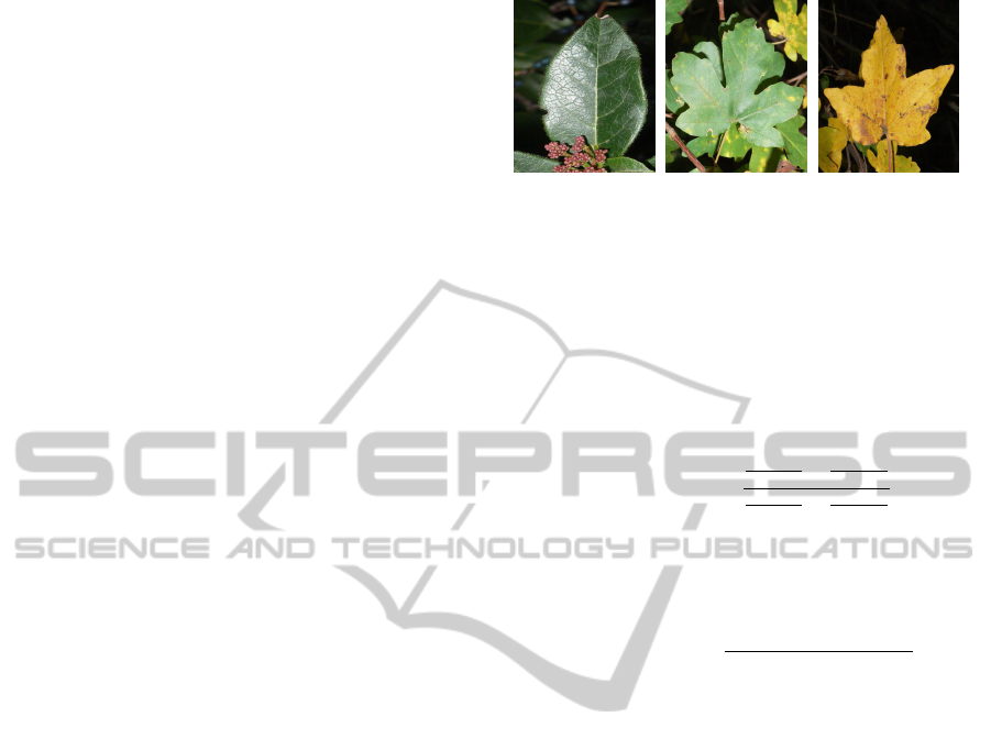
Brochier et al., 2013). Illustrated in Figure 1, this

database is composed of 232 images (from smart-

phones) of tree leaves with ground truth. They are

simple or palmately lobed leaves on plain or natural

background.

Figure 1: Sample images from the database.

To quantify the segmentation (quality, precision,

information extracted, ...), we opt for the analysis

of six observation criteria: The Dice index (or F-

measure) that characterizes the overall quality of the

segmentation area. Based on statistical tests of true

or false positives (respectivily denoted by TP and FP)

and true or false negatives (respectivily denoted by

TN and FN), the Dice index is deﬁned by:

Dice index = 2.0 ×

T P

T P+T N

T P

T P+FN

T P

T P+T N

T P

T P+FN

;

using these tests, Manhattan (or Matching) index al-

lows to study the similarity rate of the entire image,

and is deﬁned by:

Manhattan index =

T P + FP

T P + FP + T N + FN

We also study: the Hamming measure that calculates

the number of disparities between two images; the

Hausdorff distance which can be deﬁned by the max-

imum gap (in pixels) between two segmentations; the

mean absolute distance (denoted by MAD) that ana-

lyzes contour points therefore the shape of the seg-

mentation; and the structural similarity (denoted by

SSIM (Wang et al., 2004)) for the structural informa-

tion extracted.

To highlight the inﬂuence of pre-processing tools

on segmentation methods, we have chosen to compare

ten methods, referenced in Table 1. Our study is based

on : a method by Thresholding, a Watershed, two

Snakes including one using B-Splines, two versions

of MeanShift, a Graphcut, a Grabcut, Felzenswalb’s

and GAC’s algorithms. We have chosen two types of

improvement: the use of three color distance maps

and the manual initialization.

2.1 Color Distance Maps

The use of the color distance map allows the user to

enhance the contrast and therefore the contours. This

process is based on two assumptions: the object is in

the center of the image and the background is in the

corners. They are characterized by ﬁve seedpoints re-

spectively one for the center and four for the corners.

VISAPP2014-InternationalConferenceonComputerVisionTheoryandApplications

508

The principle will be to study the colors and varia-

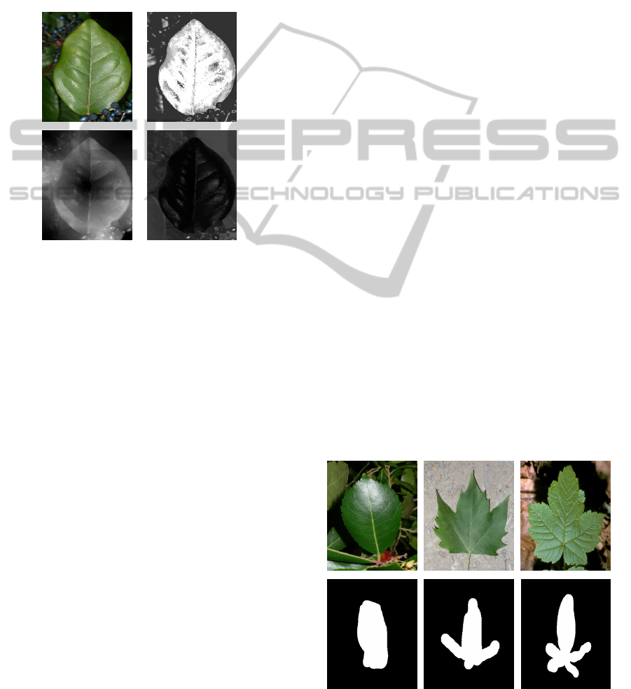
tions around these points. Figure 2 shows three types

of distance map: the ﬁrst based on coupling global

distance and local color (Cerutti et al., 2011) (denoted

by GD/LC), only using one seedpoint (in the center);

the second based on a geodesic distance (denoted by

GD), using the ﬁve seedpoints; and the last one based

on an approach of minimum barrier distance (Karsnas

et al., 2012; Strand et al., 2013) (denoted by MBD),

using a single seedpoint.

Figure 2: Sample of color distance maps: (top: left to right)

initial image, coupling global distance/local color, (bottom:

left to right) geodesic distance, minimum barrier distance.

The tool proposed by G. Cerutti (Cerutti et al., 2012)

is based on modeling the local color, deﬁned by a

distribution of a set of Gaussian. The color distance

map is therefore based on a model of global linear re-

gression, on a local adaptative mean color and on an

evidence-based combination. The dissimilarity map

is deﬁned by the distance of every pixel x in the im-

age to the color model:

LinReg

(x) = k(L

) − (L

a(L

b(L

))k

in the L*a*b colorspace. The local adaptative mean

color is based on the analysis of the 8 nearest neigh-

bours (denoted by N

) of pixel x and is deﬁned by:

∀y ∈ N

(x),A =



αB + (1 − α)C, if kB −Ck

< θ

C, otherwise

with A = (

), B = (L

) and

C = (

). The ﬁnal map is based on the

combination of the elements detailed above, ac-

cording to the theory of evidence deﬁned by Shafer

(Shaf76).

The two over color distance maps are deﬁned

on subsets space of the image points. The principle

lies in estimating the shortest distance between a

point of the object to be extracted and the back-

ground. In (Strand et al., 2013), the barrier cost

function of a path is the difference of the maximum

and minimum intensity along the path. The minimum

barrier distance between two points is deﬁned by

the barrier cost of the cheapest path with between

the points. In (Karsnas et al., 2012), the vectorial

minimum barrier distance (MBD) was introduced.

This is a method that can be used to compute distance

transforms on color images. The cost of a path π

is given by a path-cost function C ( f ,π). Let Π be

the set of all paths between p and q in (Z

,α). The

path-cost distance between p and q is

(p, q) = min

π∈Π

C ( f , π) .

The minimum barrier distance as deﬁned in (Strand et

al., 2013) is obtained by setting

C ( f , π) =



max

[ f (p

)] − min

[ f (p

)]



With the notation

f = ( f

, f

) for RGB-values, we

used the following path-cost function for color im-

ages:



f , π



∑

k=1

max

i, j



) − f

)



Note that this path cost function corresponds to the L

diameter in RGB-space of the points in the path. See

(Karsnas et al., 2012) for details.

2.2 Input Stroke

For methods permitting it, we propose to add a man-

ual stroke done with the smartphone interaction. This

input stroke, illustrated in Figure 3, allows the user

to locate the leaf in the image and to extract the local

color.

Figure 3: Sample images of tree leaves and their respective

input stroke.

AbouttheImpactofPre-processingToolsonSegmentationMethods-AppliedforTreeLeavesExtraction

509

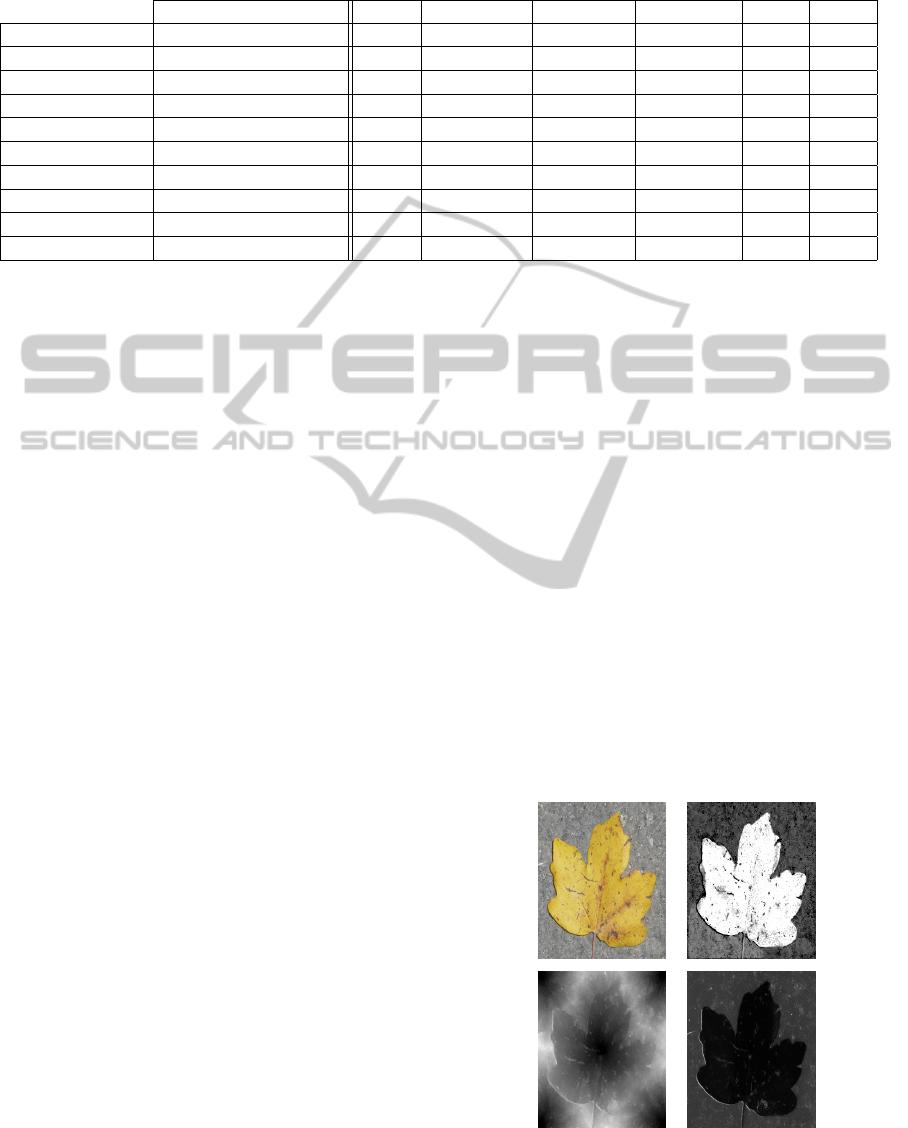
Table 1: Average Dice index, Manhattan index, Hamming measure, Hausdorff distance, MAD and SSIM of 232 images. Ten

segmentation methods are presented, with NO input stroke and with NO color distance map.

ref. Dice Manhattan Hamming Hausdorff MAD SSIM

Thresholding (Otsu, 1979) 0.751 81.27% 12969.5 80.15 6.69 0.67

MeanShift (Cheng, 1995) 0.759 81.23% 12624.8 76.57 6.31 0.70

Pyr. MeanShift (Cheng, 1995) 0.763 81.05% 13021.5 67.38 5.77 0.73

Graphcut (Boykov, 2001) 0.727 78.91% 14435.8 81.29 6.81 0.63

Watershed (Beucher, 1993) 0.749 80.14% 13594.8 74.93 6.13 0.70

Snakes (Chan, 2001) 0.735 80.43% 13060.2 80.31 5.98 0.66

B-splines Snake (Brigger, 2000) 0.809 86.70% 8692 34.3 4.20 0.77

Grabcut (Rother, 2004) 0.876 90.78% 6425.6 41.56 7.16 0.77

Felzenszwalb (Felzenszwalb, 2004) 0.686 81.80% 12474.4 38.6 4.37 0.77

GAC (Cerutti, 2011) 0.881 91.78% 4215.3 15.44 2.39 0.81

This mark also allows algorithm to have an a pri-

ori knowledge on the number of lobes composing the

leaf (simple or palmately lobed).

3 RESULTS AND DISCUSSION

In this paper, we propose to study successively the

performance of segmentation methods, without pre-

processing, then with a distance map, of which we

present optimizations, and ﬁnally with the addition

of a manual initialization. The number of results is

quite substancial, so we opt for a comparative analy-

sis based on mean values obtained by each approach

on the 232 images. For methods using thresholds or

adjustable parameters, we present in this paper the

best results obtained after optimization of these ap-

proaches with a collection of images.

3.1 With no Initialization and with no

Color Distance Map

First, we present in Table 1, the performance ob-

tained by each segmentation methods without prepro-

cessing tools. We see a very clear superiority of the

Guided Active Contour approach, for the problem of

tree leaves segmentation. Indeed, quality of segmen-

tation (given by the Dice index) is increased by 12%.

The Manhattan index, characterizing the problems

of sub- and over-segmentation, is also improved by

nearly 8%. The Hamming measure conﬁrms the pre-

vious observations, since the average number of dis-

similarities is divided by 2.5. The Hausdorff distance

provides precision on dispersion of the segmented re-

gions. Indeed, guided active contour shows an aver-

age value equal to 15.44 pixels while the conventional

methods get much higher values. The two last crite-

ria (MAD and SSIM) are used to analyse the shape of

the segmentation as well as the quality of information

extracted according to the ground truth, through struc-

tural analysis. GAC method improves the shape of the

segmentation by a factor 3, and the structural aspect

is increased by 8% compared to the other approaches.

3.2 With no Initialization and with

Color Distance Map

The idea is to replace the original images with more

contrast images to facilitate and improve the segmen-

tation. The results presented in Tables 2,3 and 4 are

based on three types of color distance maps. The ﬁrst

observation concerns the performance offered by the

methods for each of the color distance maps. Indeed,

for a problem of segmentation of tree leaves, it ap-

pears that the use of a coupling global distance and lo-

cal color provides the best results. This observation is

conﬁrmed by Figure 4, which shows the limits of the

other two colors distance map algoritms in the case of

natural background. The second observation relates

to the improvement in term of performance given to

Figure 4: Color distance maps: (top: left to right) initial

image, coupling global distance/local color, (bottom: left to

right) geodesic distance, minimum barrier distance.

VISAPP2014-InternationalConferenceonComputerVisionTheoryandApplications

510

Table 2: Average Dice index, Manhattan index, Hamming measure, Hausdorff distance, MAD and SSIM of 232 images.

Ten segmentation methods are presented, with NO input stroke and with color distance map based on coupling global

distance and local color.

ref. Dice Manhattan Hamming Hausdorff MAD SSIM

Thresholding (Otsu, 1979) 0.855 89.51% 7176.8 48.72 5.87 0.78

MeanShift (Cheng, 1995) 0.816 86.35% 9980.1 61.42 5.56 0.72

Pyr. MeanShift (Cheng, 1995) 0.846 88.33% 8055.5 51.08 5.11 0.78

Graphcut (Boykov, 2001) 0.79 85.46% 10220.2 63.13 6.09 0.69

Watershed (Beucher, 1993) 0.82 84.93% 11624 62.66 5.35 0.76

Snakes (Chan, 2001) 0.834 87.58% 9251.1 63.57 5.24 0.75

B-splines Snake (Brigger, 2000) 0.864 90.42% 6432.7 30.9 3.78 0.80

Grabcut (Rother, 2004) 0.789 83.52% 9397.5 50.08 6.80 0.72

Felzenszwalb (Felzenszwalb, 2004) 0.793 86.70% 8246.2 34.57 3.81 0.79

GAC (Cerutti, 2011) 0.903 94.06% 3780.9 11.56 1.56 0.86

Table 3: Average Dice index, Manhattan index, Hamming measure, Hausdorff distance, MAD and SSIM of 232 images. Ten

segmentation methods are presented, with NO input stroke and with color distance map based on geodesic distance.

ref. Dice Manhattan Hamming Hausdorff MAD SSIM

Thresholding (Otsu, 1979) 0.653 78.66% 13465.2 41.90 11.32 0.72

MeanShift (Cheng, 1995) 0.647 77.49% 13861.4 42.64 10.49 0.72

Pyr. MeanShift (Cheng, 1995) 0.619 75.19% 14566.1 47.61 11.44 0.71

Graphcut (Boykov, 2001) 0.621 77.72% 13921.5 40.81 12.30 0.69

Watershed (Beucher, 1993) 0.655 77.80% 13649.3 42.97 11.94 0.72

Snakes (Chan, 2001) 0.648 80.07% 12766.1 35.35 13.46 0.73

B-splines Snake (Brigger, 2000) 0.673 67.23% 21863.4 71.34 7.43 0.73

Grabcut (Rother, 2004) 0.639 61.08% 22364.0 64.32 6.87 0.61

Felzenszwalb (Felzenszwalb, 2004) 0.664 64.86% 23621.7 72.55 6.29 0.64

GAC (Cerutti, 2011) 0.788 84.32% 5396.8 17.63 4.28 0.78

Table 4: Average Dice index, Manhattan index, Hamming measure, Hausdorff distance, MAD and SSIM of 232 images. Ten

segmentation methods are presented, with NO input stroke and with color distance map based on minimum barrier

distance.

ref. Dice Manhattan Hamming Hausdorff MAD SSIM

Thresholding (Otsu, 1979) 0.539 55.19% 32052.2 100.36 9.52 0.70

MeanShift (Cheng, 1995) 0.563 56.59% 30082.2 89.57 8.97 0.68

Pyr. MeanShift (Cheng, 1995) 0.560 57.55% 28861.3 88.06 8.68 0.65

Graphcut (Boykov, 2001) 0.54 57.90% 29782.3 96.22 10.34 0.68

Watershed (Beucher, 1993) 0.541 51.91% 35039.5 101 8.40 0.67

Snakes (Chan, 2001) 0.59 72.58% 15137.3 31.19 16.3 0.71

B-splines Snake (Brigger, 2000) 0.561 56.59% 30082.1 89.57 8.97 0.73

Grabcut (Rother, 2004) 0.592 47.21% 36216.4 88.02 10.84 0.50

Felzenszwalb (Felzenszwalb, 2004) 0.627 53.61% 34599.1 87.44 9.07 0.57

GAC (Cerutti, 2011) 0.728 80.44% 8245.2 23.01 6.16 0.77

segmentation approaches. By analyzing Table 2, we

can highlight a signiﬁcant increase in all observation

criteria. From a general point of view, the results im-

proved by nearly 10%. In the case of Guided Ac-

tive Contour method, we notice 2.5% improvement

for the Dice and Manhattan index. The average num-

ber of dissimilarities (Hamming measure) and Haus-

dorff distance are reduced respectively by 11.5% and

33.6%. The shape of segmentation (MAD) and textu-

ral information extracted (SSIM) were also increased

respectively by 53.2% and 6.5%.

To achieve this performance, different tests were

applied to determine the best possible color dissim-

ilarity. We proposed a comparative analysis of the

distance to the average color based on: a Gaussian,

a linear regression, a local mean and a combination

AbouttheImpactofPre-processingToolsonSegmentationMethods-AppliedforTreeLeavesExtraction

511

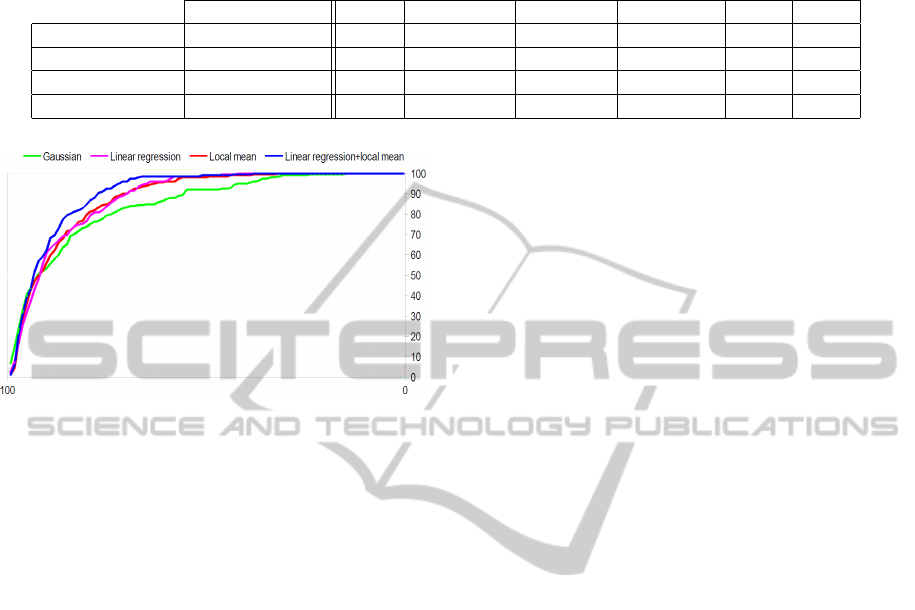
Table 5: Average Dice index, Manhattan index, Hamming measure, Hausdorff distance, MAD and SSIM of 232 images. Four

segmentation methods are presented, with initial trace and with color distance map based on coupling global distance

and local color.

ref. Dice Manhattan Hamming Hausdorff MAD SSIM

Snakes (Chan, 2001) 0.872 91.43% 6094.2 40.92 5.12 0.67

B-splines Snake (Brigger, 2000) 0.861 90.67% 6211.7 29.13 3.45 0.79

Grabcut (Rother, 2004) 0.898 92.46% 4931.5 35.55 6.44 0.85

GAC (Cerutti, 2011) 0.927 95.45% 2872.7 10.82 1.06 0.87

Figure 5: Recovery rate depending on the value of recovery

for four color distance estimations.

of linear regression/local mean. Figure 5 shows a plot

of recovery rate depending on the value of recovery.

Given the results, we therefore opted for color dis-

tance maps based on combination of linear regression

and local mean for all of our tests presented in this

paper.

3.3 With Initialization and with Color

Distance Map

The second improvement is based on the interaction

between the user (via a smartphone for example) and

the algorithm. For methods allowing it (Snakes, B-

splines Snake, Grabcut and Guided Active Contour),

we integrate an initial trace to locate and retrieve the

local color of the leaf. Table 5 presents performances

obtained for the four approaches coupled with an ini-

tial trace. The best of them, the GAC method, has in-

creased its Dice index and Manhattan index by 2.5%.

It has a Dice index greater than 92%, representing

therefore a very good result in terms of precision.

The quality of the segmentation has been improved

through the Hamming measure and the Hausdorff dis-

tance, reduced respectively by 31.6% and 6.8%. The

segmentation area is better deﬁned, the MAD is in-

crease by 47.1%, thus approaching an average offset

of 1 pixel, and the SSIM shows that information ex-

tracted corresponds more to the ground thruth, with a

rate close to 0.9.

3.4 Illustration

To visualize the different improvements achieved

through pre-processing tools, we propose some illus-

tration in Figures 6 and 7. For better clarity, we re-

strict ourselves to one approach with problem of seg-

mentation and one other approach with the best re-

sults. In view of all the results, it appears that the

method developed by Cerutti (Cerutti et al., 2011),

coupled with a distance map based on the coupling

global distance/local color and an initial trace, has

the best performance for almost all images of the

database.

4 CONCLUSIONS

We have presented in this paper a comparative study

of the inﬂuence of pre-processing tools on segmenta-

tion methods. Our analysis focuses on the challeng-

ing problems of extracting tree leaves on natural back-

ground. We propose at ﬁrst the use of color distance

map, in particular the coupling global distance and lo-

cal color, to increase signiﬁcantly the performance of

all the tested approaches. Subsequently, we added an

initial trace for methods permitting it, relying on tech-

nological developments and user needs. Ultimately,

these tools have enabled us to improve the precision,

shape and quality of the information extracted, in par-

ticular for the Guided Active Contour method. This

method also provides a more stable segmentation, as

we detailed in (Grand-Brochier et al., 2013), through

the study of standard deviations, which are lower for

all observation criteria. These improvements result in

increased computation time, remaining nevertheless

acceptable in relation to the proposed performance:

around 3.5sec per segmentation against 0.09sec for

Thresholding, 1.5sec for Snakes and 60sec for B-

spline snake.

In terms of prospects, we are currently studying

other tools to reduce potential problems of sub- or

over-segmentation. We also wish to study the inﬂu-

ence of the pre-processing tools on the description

and classiﬁcation steps. We are also considering the

VISAPP2014-InternationalConferenceonComputerVisionTheoryandApplications

512

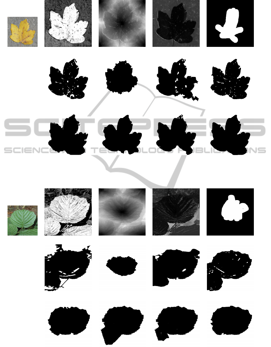
initial image GD/LC GD MBD stroke + GD/LC

B-splines Snakes approach (Dice index (left to right): 0.829, 0.412, 0.618 and 0.871)

Guided Active Contour approach (Dice index (left to right): 0.901, 0.855, 0.820 and 0.948)

Figure 6: Segmentation obtained for distance maps based on (left to right) : coupling Global Distance/Local Color, Geodesic

Distance, Minimum Barrier Distance, and GD/LC with input stroke, for B-splines Snakes and GAC approaches.

initial image GD/LC GD MBD stroke + GD/LC

Grabcut approach (Dice index (left to right): 0.682, 0.479, 0.623 and 0.704)

Guided Active Contour approach (Dice index (left to right): 0.914, 0.813, 0.836 and 0.951)

Figure 7: Segmentation obtained for distance maps based on (left to right) : coupling Global Distance/Local Color, Geodesic

Distance, Minimum Barrier Distance, and GD/LC with input stroke, for Grabcut and GAC approaches.

AbouttheImpactofPre-processingToolsonSegmentationMethods-AppliedforTreeLeavesExtraction

513

implementation of an application bringing together all

this benchmark, in order to use it on any kind of do-

main (medical imaging, object tracking, or any other).

We are currently developing a site for online voting,

to test different methods of segmentation with differ-

ent pre-processing tools and analyze, from a statistical

viewpoint, the results through a panel of 24 observa-

tion criteria.

REFERENCES

Beucher S. and Lantujoul C. (1979). Use of watersheds in

contour detection. REMD.

Beucher S. and Meyer F. (1993). The morphological ap-

proach to segmentation: the watershed transforma-

tion. MMIP, p. 433-481.

Boykov Y. and Jolly M. (2001). Interactive graph cuts for

optimal boundary and region segmentation. ICCV,

vol. 1, p. 105-112.

Brigger P. et al. (2000). B-spline snakes: a exible tool for

parametric contour detection. Trans. on Image Pro-

cessing, vol. 9(9), p. 1484-1496.

Canny J. (1986). A computational approach to edge detec-

tion. PAMI, vol. 8(6), p. 679-698.

Cerutti G. et al. (2011). Guiding Active Contours for Tree

Leaf Segmentation and Identiﬁcation. CLEF.

Cerutti G. et al. (2012). ReVeS Participation - Tree Species

Classiﬁcation Using Random Forests and Botanical

Features. CLEF.

Chan T. and Vese L. (2001). Active Contours Without

Edges. Trans. on Image Processing, vol. 10(2), p. 266-

277.

Cheng Y. (1995). Mean Shift, Mode Seeking, and Cluster-

ing. PAMI, vol. 17(8), p. 790-799.

Felzenszwalb P. and Huttenlocher D. (2004). Efﬁcient

Graph-Based Image Segmentation. IJCV, vol. 59(2),

p. 167-181.

eau H. et al.. (2011). The clef 2011 plant images classi-

ﬁcation task.

Grand-Brochier M. et al. (2013). Comparative Study of

Segmentation Methods for Tree Leaves Extraction.

VIGTA, vol. 7.

Greig D.et al. (1989). Exact maximum a posteriori estima-

tion for binary images. JRSS, vol. 51, p. 21-279.

Horowitz S. and Pavlidis T. (1974). Picture segmentation by

a directed split and merge procedure. ICPR, p. 424-

433.

Horvath J. (2006). Image segmentation using fuzzy c-

means. SAMI.

Karsnas A. et al. (2012). The vectorial Minimum Barrier

Distance. ICPR, p. 792-795.

Kass M. et al. (1987). Snakes : Active contour model. IJCV,

p. 321-331.

Kumar N. et al. (2012). Leafsnap: a computer vision sys-

tem for automatic plant species identiﬁcation. ECCV,

2012, p. 502-516.

Kurtz C. et al. (2010). Multiresolution region-based clus-

tering for urban analysis. IJRS, vol. 31(22), p. 5941-

5973.

Lynch M. et al. (2006). Automatic segmentation of the left

ventricle cavity and myocardium in MRI data. CBM,

vol. 36(4), p. 389-407.

Malmberg F. et al. (2012). Smart Paint - A New Interactive

Segmentation Method Applied to MR Prostate Seg-

mentation. MICCAI.

Marr D. and Hildreth E. (1980). Theory of Edge Detection.

Biological Sciences, vol. 207(1167), p. 187-217.

Neto J. et al. (2006). Individual leaf extractions from young

canopy images using Gustafson-Kessel clustering and

a genetic algorithm. CEA, vol. 51(1), p. 66-85.

Otsu N. (1979). A threshold selection method from gray-

level histograms. TSMC, vol. 9(1), p. 62-66.

Rother C. et al. (2004). ”Grabcut”: interactive foreground

extraction using iterated graph cuts. SIGGRAPH, p.

39-314.

Salman N. (2006). Image segmentation based on watershed

and edge detection techniques. IAJIT, vol. 3(2), p.

104-110.

Shafer G. (1976). A Mathematical Theory of Evidence.

Princeton University Press.

Strand R. et al. (2013). The minimum barrier distance.

CVIU, vol. 117(4), p. 429-437.

Teng C. et al. (2011). Leaf segmentation, classiﬁcation, and

three-dimensional recovery from a few images with

close viewpoints. Opt. Eng., vol. 50(3).

Valliammal N. and Geethalakshmi S. (2012). Plant Leaf

Segmentation Using Non Linear K means Clustering.

IJCSI, vol. 9(1), p. 212-218.

Wang S. and Haralick R. (1984). Automatic multithreshold

selection. CVGIP, vol. 25, p. 46-67.

Wang Z. et al. (2004). Image quality assessment: From

error visibility to structural similarity. TIP, vol. 13(4),

p. 600-612.

Zimm C. et al. (2002). Segmentation and tracking of mi-

grating cells in videomicroscopy with parametric ac-

tive contours: a toll for cell-base drug testing. Medical

Imaging, vol. 21(10), p. 1212-1221.

VISAPP2014-InternationalConferenceonComputerVisionTheoryandApplications

514